Remember, you are required to read the blog at least once per day. Usually I will also send an e-mail note announcing that I've made a new blog post.
Wednesday, March 23, 1945Please note that I have a Web page detailing my policy regarding letters of recommendation. I revised it substantially just now. You may find it valuable even if you do not intend to ask me for a letter.
Wednesday, March 23, 1020All done! Grades submitted to the Registrar. They show up on the faculty Registrar site, so I assume they are visible to you on Canvas. Let me know if not.
Tuesday, March 22, 2235Sorry for the delay in course grades, which was due mainly to grading ECS 188, putting out fires in both classes (major issue: wrong e-mail addresses on exams, hwk etc.), and some personal tasks, e.g. dental appointment. I also had to rewrite my grading scripts somewhat, for various reasons.
At any rate, everything is all set to go. I'll run the final script tomorrow morning, midday at the latest. You should be able to figure out your course grade from the formula percentages (in some cases, a grade may be bumped up somewhat), but if you wish confirmation before I send out the grades, feel free to contact me.
Sunday, March 20, 2235I have now finished grading the projects. Overall they were good. There were a couple of A+ projects, and several others of A+ quality except for failure to follow specs, which got A grades instead. The lowest project grade was B-; three groups had this grade.
For each project, I have not only a grade but also notes. If you wish to see these, feel free to e-mail me. I'd be happy to show them to you.
I hope to get the course grades out tomorrow night.
Saturday, March 19, 2150Hi, everyone. It will be at least 2 more days before I will have your Term Project grades ready. Sorry for the delay.
Thursday, March 17, 1340HUGELY IMPORTANT REMINDER: All your course records are indexed by your official UCD e-mail address. This is the address I've been using to e-mail you with. If the Term Project file your group submitted yesterday was incorrect (e.g. 'jsmith' rather than 'jbsmith', the records will show that YOU DID NOT DO THE TERM PROJECT. I try to watch out for these things, but there is no guarantee.
So, check the exact name of the .tar file your group submitted. If it was incorrect, CONTACT ME IMMEDIATELY.
Wednesday, March 16, 2005Remember to submit your partial work at least once, in order to ensure that you've at least submitted something, and in order to make sure you are properly submitting to my (not Stefan's) handin site. (Your later submissions will overwrite the earlier ones.) If you have any trouble submitting, please e-mail both Stefan and me.
Wednesday, March 16, 0950Please note that I will be PRINTING your reports for grading. That means the axes, labels etc. must be readable in that size.
Monday, March 14, 1525Please recall this part of the Term Project requirements:
Progress report: Due Monday, March 14, 11:59 pm, in the form of an e-mail message to me. Must be a frank discussion stating the contribution of each group member so far.Saturday, March 12, 2255
If you have been using the new function qeParallel() to speed up your code, recall that I said it had a few rough edges (though certainly usable). I've worked a bit on that, simplifying the interface.
Example of new argument format:
qeParallel(pef,'wageinc','qeRF','pef',
   cls=2,libs='randomForest',opts='nTree=100',holdout=1000)
Should get a man page out tomorrow, but the new argument roles should be clear. See the comments in the source code for more details if needed.
Saturday, March 12, 1035In order to make sure we are all "on the same page" re the Term Project, I asked Stefan to write a summary of the goals. Since his phrasing is different from mine, this gives you an independent "second opinion," again just to make sure you are on the right track. I'm enclosing his summary here. Hopefully, as you read it, you will be thinking, "Yes, this is consistent with what we are doing..."
The goal of the project is to run a semi-comprehensive analysis on some of the factors that affect the accuracy of a model. We've spent a large part of the quarter looking at how features can affect accuracy, but features aren't the only variable in a recommender system. The characteristics of the data play a large role as well. For this project, the characteristics you'll be looking at are the number of users, the number of items, and the number of non-missing values (the density). Like any good scientific experiment, to tease out the effect of each factor, you're going to hold everything but that factor constant and see how/if the outcome changes. You're likely more familiar with this approach in the context of chemistry, physics, or biology experiments, but it can be applied to any scientific inquiry. To begin, you'll want a "fully populated" dataset, i.e., one with a rating for every user/item pair (to understand why this is the case, you can read the blog post from Tuesday, March 8, 1400). Since real world datasets are almost never this dense, your first step after choosing a dataset will likely be filling in the missing values using the modeling technique of your choice. This fully dense dataset is the "aEst" that Dr. Matloff is referring to in the project description and his blog posts. Once you have your aEst, you can begin your controlled experiments. How well does a model trained on aEst perform when the number of users changes but everything else is held constant? What about when only the number of items changes? Does introducing NAs affect performance? Are the trends the same for matrix factorization (MF) and non-MF techniques?Saturday, March 12, 1000
PLEASE TAKE IMMEDIATE ACTION if you did not receive your Group Quiz grade, in the mailing I sent out earlier this morning. The likely cause is one of the following, concerning your group member who submitted your Group Quiz:
Again, please contact me IMMEDIATELY if you did not receive your Group Quiz grade. Please recall the blog post of February 25, 1500:
The Group Quiz will be collaborative among your group members. The collaboration will be noisy and hopefully fun. All group members must be physically present; any missing member will get an F on the quiz, as well as a major penalty on the course grade. The latter is also true if a group member clearly has not participated much in a homework assignment or the term project.Saturday, March 12, 0945
The grades on the Group Quiz were generally good:
> table(z[,7])

 A A+ A- B+ B-  C  F
 2 10  7  8  4  3  6
Remember, under the revised grading system, your Quiz grade will be the average of your top three letter grades on the Quizzes. The other day in class, I predicted that for many students, the Group Quiz will be among their top three, and the above results would seem to confirm this.
So...in spite of all the tumult during the quarter, I believe that most of you will end up with a good, solid course grade, in the A or B range.
Make sure you support this with a good solid Term Project. I'd be happy to take a look at your draft report to confirm that it is doing what is needed. As I said before, time will not permit me to read the draft in detail, but I can glance through it enough to be able to confirm that you are on the right track.
Note that a Progress Report is due this Monday.
Thursday, March 10, 2245The new qeML parallel computation function is now ready for download (qeML version 1.0.1). It still has some rough edges, but definitely usable, and can really speed things up. Here is an example:
> system.time(qeSVM(pef,'occ',holdout=1000))
holdout set has  1000 rows
Loading required package: e1071
   user  system elapsed
 99.650   0.044  99.723
> system.time(qeParallel("nodeCmd=qeSVM(pef,'occ',holdout=NULL)",
   cls=4,dataName='pef',yName='occ',holdout=1000))
Loading required package: partools
Loading required package: parallel
Loading required package: data.table
data.table 1.14.0 using 4 threads (see ?getDTthreads).  Latest news:
r-datatable.com
holdout set has  1000 rows
   user  system elapsed
  1.076   0.016   9.643
More than a 10-fold speedup! This is called superlinear, as it came from only 4 threads. The theory in my JSS paper, linked to earlier in the blog, shows why this can happen.
The theory also shows that the accuracy should be the same, whether in the original serial (i.e. non-parallel) version or via qeParallel().
How did the arguments work above?
A real cluster, say on CSIF, could be set up via a character vector, e.g.
c('pc21', 'pc22', 'pc23', 'pc24', 'pc25', 'pc26', 'pc27', 'pc28')
In fact, by listing each node twice, say, we could potentially get a degree of parallelism of 16, and maybe much more, though there is also a "law of diminishing returns" for parallelism.
One "rough edge" is that you may need to load the underlying library manually, e.g.
library(randomForest)
If you try this, please let me know of any questions or problems that arise.
Note too that rectool::xvalReco() also has a 'cls' argument. It works as above, but you must create the cluster yourself, e.g.
cls <- makeCluster(4) # 4 coresThursday, March 10, 1330
Tomorrow's Group Quiz will consist pf two problems. I consider the first to be the more important of the two, and as such, I will guarantee that if you get it completely correct, your Quiz grade will be at least A-. This problem will ask you to implement a function that I will probably add to rectools later.
The second problem involves writing some code that implements a certain matrix operation.
Wednesday, March 9, 1945Function arguments that are themselves functions:
This is something you should have seen somewhere along the way, e.g. with the qsort() function in the C library. Here is an excerpt from the man page:
void qsort(void *base, size_t nmemb, size_t size,
      int (*compar)(const void *, const void *));
That fourth argument is a function, with the formal argument name compare(). Sorting numbers is easy, but what if we want to sort character strings? How do we decide how to compare two strings? This function defines it.
There are tons of examples in R and Python. Even the mundane R apply() function is one:
> args(apply)
function (X, MARGIN, FUN, ...)
Wednesday, March 9, 1940
Re the Term Project: Say you tell a friend about the project, who asks, "Why not just look at several different real sets, to see the effects of varying n, m and p?" How would you answer?
One of the major educational benefits of this project, beyond its speciic recommender systems content, is the design of a controlled experiment. Not only is this part of an engineering education, but it also is important to understand as an educated person. E.g. when the newspaper talks of a Randomized Clinical Treatment study of a new medical procedure, you should have some idea of what this means.
In that sense, you should not be asking me "What should be in the outer loop and what in the inner loop?" kinds of questions. Instead, ask yourself how to design your experiments in a meaningful, convincing way.
Wednesday, March 9, 1425The material from today's lecture is at the usual URL,
Wednesday, March 9, 0825Group Quiz on Friday!
R's get() function can come in very handy when writing general code intended for use by many different people. Given the name, it gives you the object:
> x <- 8
> z <- get('x')
> z
[1] 8
But even object names are in essence pointers internally:
> x <- 3
> z
[1] 8
Here z did not change when x did. The latter had been pointing at (a memory location containing) 8, but we changed it to point to 3; z is still pointing to 8.
Tuesday, March 8, 1400For (my suggested approach) to the Term Project, you might find it helpful to think of what could be done instead, if the project were not required to vary d, in terms of generating synthetic data frames.
E.g. we could use the MovieLens data as follow. To keep m (number of movies) fixed, we could randomly choose m of the 1682 movies, then reduce the data frame to only records involving those m movies. Let's call this data frame DFm. Then say we want to consider what happens with n = 100, n being the number of users. We could randomly choose n of the users in the reduced data frame, and then use records only involving those n users. Call this data frame DFmn We could then use Recosystem or whatever on DFnm. Then say we want to try n = 250, but with the same m. We now choose 150 users from DFm, etc. In this manner, we would be varying n while keeping m fixed.
But this would be difficult if we also need to vary d, which we do. The d in DFm is probably different from the d in the full data. Thus we will have varied both m and d, violating our requirement that we vary one quantity at a time.
With my suggested approach, we first get a completely intact synthetic ratings matrix. We vary m by taking the first m columns, or n by taking the first n rows. We vary d by varing the amount of NAs we sprinkle in. Most important, we can vary any one of these quantities while holding the other two fixed.
Once we get the portion of the ratings matrix corresponding to our n and m, and have done the sprinkling for d, then we call toUserItemRatings() to convert to input matrix form. That will be the data we run our various methods on, whether it be Recosystem, the linear model or whatever
Tuesday, March 8, 1035The toUserItemRatings() function requires row and column names in the ratings matrix. I've now added a check for that.
The function toRatingsMatrix() automatically creates row and column name. As it is meant to be paired with toUserItemRatings(), I've now removed buildMatrix(); use toUserItemRatings() instead.
I've updated the man pages for these functions accordingly.
Again, you won't need these functions in the Group Quiz, but they will be needed in your Term Project.
Monday, March 7, 1645Topic: PARALLEL COMPUTATION IN R!
A conversation with some students in my office hour today revealed yet another Machine Learning Rumor--R does not do parallel computation, and Python ML does. This really shocked me. It's totally false! Parallel computation is actually vital to serious R users. In fact, I wrote a book about it. Here are some specifics:
First, since so much of R is matrix-based, a very powerful way to get multihreaded computation in R is to use a multihreaded BLAS (Basic Linear Algebra Subroutines). There is a default BLAS that your R binary was built on, but it's better to build from scratch (the standard 'configure; make; make install' sequence familiar to CS majors), using Open BLAS instead of the standard BLAS. See this blog post. You then get multithreaded operation automatically on anything you do with matrices in R.
Second, there is a general parallelization method that works well on any machine learning algorithm, known variously as bagging, chunk averaging and my own term, Software Alchemy, as follows:
First think of random forests, say with 500 trees. We generate 500 trees from our training data, and then when we have a new case to predict, we plug it in to each tree, giving us 500 predicted values. We then average those 500 values to give us our final prediction.(If Y is categorical, then we take a "vote" among the 500 tree decisions. Whichever category "wins," that is our overall decision.)
Well, the point is that if we want to do this in parallel, across say 4 cores, we simply have each core generate 500/4 = 125 trees, thus giving us 500 trees. We still take the average of 500 trees, either way.
For something like SVM (to be covered on Wednesday), we can split our data randomly into 4 chunks, and run SVM on each. Faced with a new case to predict, we get 4 predictions, then either average or "vote" on the results to get our overall prediction.
In fact, this is done in SciKit-Learn's SVM , indeed under the name of "bagging."
Granted, SciKit-Learn offers you that option, rather than in R you must arrange the bagging yourself. But if you wish to use formal structure for it, there are routines in my partools package.
What's interesting is that not only can one get parallelism from bagging, one may attain superlinear speedup, i.e. a speedup of greater than c for c cores. See the details here.
Monday, March 7, 0825I've fixed a couple of things in toRatingsMatrix() and toUserItemRatings(). If you use these functions in your project (they won't arise in the Group Quiz), be sure to use rectools 1.1.4 or higher.
Saturday, March 5, 1105Yesterday in lecture I gave some tips for preparing for the Group Quiz (March 11, 9-10 am, Hoagland 168). Here is a somewhat expanded version:
> scramble <- sort
> x <- c(5,12,13,8,88)
> sort(x)
[1]  5  8 12 13 88
> scramble(x)
[1]  5  8 12 13 88
> f
function(x,sortFtn) {
   sortFtn(x)
}
> f(x,sort)
[1]  5  8 12 13 88
> f(x,scramble)
[1]  5  8 12 13 88
Several people asked me after class yesterday about the details of random forests. I had not intended to go into detail, just sticking with presenting the "flow chart" nature of RFs. But I've now added some material on that, which also corrects an error. (The original version said that Node 7 was left intact in the tree building process, which is not true.)
Thursday, March 3, 1705The material on decision trees and random forests is now ready in our text.
Wednesday, March 2, 2000It's really important that you have a firm understanding of the goals (and suggested approach) of the problem in the term project. Here is some material that should help.
Suppose we are investigating the economic impact of Covid-19. For instance, instead of having kids learn via remote instruction in K-12, what if they attended class in-person, say in heavily fortified settings (plexiglas shields between the desks, weekly testing etc.). What would be the effects on unemployment rates, child poverty, etc.?
Well, we can't "replay" the last two years. So, we must investigate using synthetic (AKA fake) data. We could start with the real data of 2020, then develop some simulation models (too elaborate to discuss here) for how things would evolve over time. We could control for various quantities, e.g. number of kids in school, running the simulation once for each scenario of interest. In this way, we could address our various "What if...?" questions.
In the above approach, we would at least start with real data. But we could base our analysis on purely simulated data, as we did in our investigation of p-hacking, in the blog entry Thursday, February 3, 2120. There we just said, "OK, say we have data coming from some multivariate normal distribution. How much effect would p-hacking have?" And note that while we had n = 50, p = 2 in that analysis, we could vary n and p, exploring how p-hacking might work. With n much larger than p, for instance, we might find that p-hacking has very little impact.
You could do the same thing in your term project, by assuming some kind of multivariate distribution for n, m and d. It would be quite hard to think of a reasonable distribution, though, so a better approach would be the one I suggest in the specs:
Start with a real dataset, say MovieLens. Apply some collaborative filtering method, say the linear model or matrix factorization. Now you have the estimated/completed ratings matrix, aEst. Now pretend that that is a real ratings matrix from some data that originally had no NAs. Now artificially add some NAs, in proportion 1-d. At this point you can explore how good our predictive ability would be on such data, for various values of n and m. For n = 500 and m = 75, say, take the 500 x 75 "northwest corner" of aEst, thereby simulating what would happen if our n and m values were only 500 and 75. We can easily vary n and m that way; to vary d, we need to go back to the pre-sprinkling version of aEst.
In pseudocode, your experiments might look like this:
for ds in some real datasets
   form aEst from ds
   for d in some values of interest
      add some NAs to aEst, assigning to aEstSprinkled
      for n,m in some values of interest
         take the NW n x m corner of aEstSprinkled, assign to anm
         convert anm to data frame form dff
         for various RS methods of interest rsm
            apply rs to diff, with replicMeans, to see prediction accuracy
Don't lose sight of the ultimate goal: Your conclusions from your experiments would be statements like, "For n and m equal to 500 and 100, changing d makes a big difference. The graph of accuracy against d declines briskly. On the other hand, with d = 0.8 and n = 500, as m increases the graph again declines, but more slowly. Eventually, we see an effect like the Law of Diminishing returns."
Wednesday, March 2, 1645IMPORTANT NOTE: Our Group Quiz, March 11, will be held during 9-10 in Hoagland 168. We will not meet 10-11.
Tuesday, March 1, 2315Tomorrow I will begin Chapter 8 in our text, on the use of nonparametric machine learning methods in RS.
Tuesday, March 1, 0950Important notes:
In the matrix factorization chapter in our text I've added material to Sections 6.3.5 (Predicting New Cases) and 6.5 (Alternating Least Squares (ALS)).
For Quiz 7:
I've added some more detail in the Term Project specs, on how you might vary one quantity with the other two fixed.
Sunday, February 27, 1930Fixed the xvalReco() bug.
Sunday, February 27, 1710Well, I can hardly complain about liberal A+ grades and too many P/NPs in the department when my own software is causing you problems. :-) There is a bug in xvalReco(), which I actually discovered the othewr day but forgot to fix. (It's related to our being halfway into allowing covariates.) I'll fix it this evening when I get to a computer. (You may wish to fix it yourself, easy task.)
Sunday, February 27, 1625I added a function toRatingsMatrix() to rectools. It is similar to buildMatrix() but retains the original ID factor values as row and column names in the resulting matrix.
Sunday, February 27, 1555Here is an example of pre-adjustment for covariates:
lmout <- qeLin(ml100kpluscovs[,-c(1,2)],'rating',holdout=NULL)
preds <- predict(lmout,ml100kpluscovs[,-c(1,2,3)])
ml100kpluscovs$rating <- ml100kpluscovs$rating - preds
# then do one's intended rec sys analysis on this new data, remembering
to add preds back at the end
As I've mentioned, use of covariates may or may not be helpful. If a user in our dataset has rated many items, this already tells use a lot about this user's taste and preferences. Thus it may give us all the information we need for this user, with covariates adding little or nothing.
Covariates will thus be most helpful for users from whom we have very few ratings.
BTW, even though I have deleted the requirement to use softImpute(), it is still to your advantage to submit your work on it. Remember, Stefan will give A+ grades for especially good submissions (accompanied by comparably good performance in interactive grading).
Sunday, February 27, 1445Unfortunately, the docs are ahead of the code re xvalRecor(). It was a planned addition. You'll need to manually subtract the linear model predicted values from the ratings. Sorry, my bad.
Sunday, February 27, 1400I see that some groups are still stuggling with softImpjte(). I will thus drop the requirement that you use it in Problem 2; you can still get an A grade on that problem even if you omit it.
Concerning recosystem, I hope everyone is using rectools::xvalReco() for convenience.
Sunday, February 27, 1240As you all know, I was profoundly shaken earlier this quarter in finding that some quizzes had very high proportion of D and F grades. I have taught this course twice under an ECS 189G label in the past and nothing like that ever happened. So again this really profoundly affected me.
It was also troubling that one student in our class remarked that a course in a CS Dept. should not have so much math; it should just be about programming, the student said. I'd really like to know where the student got this impression, which is absolutely incorrect. Recall that I showed everyone the Web page of an undergrad machine learning class at UCB that is far more mathematical than our rec sys class; this is typical in CS Depts. across the nation.
Apparently I am not the only one who is baffled and worried. Another professor in our department gave a midterm last week in which one third of the students did not even show up for the exam! It's probably no coincidence that that class was also mathematical in nature.
I have speculated on the causes, such as an alarming proliferation of A+ grades in our courses.
After frankly stating that I have been profoundly shaken by all this, some students expressed sympathy for me. I truly appreciate this.
But whatever the cause is, here we are. Therefore I as you also know have changed the grading system dramatically to de-emphasize the quizzes.
Another remedy was that on Quiz 6, I said that most of the questions would come from page 81. In fact they all did. That was intended to allow students to really focus, rather than being distracted by the myriad different aspects of the course.
That remedy was moderately successful. It really helped some students who had been struggling. However, some others apparently did not realize that I might actually have you implement some things in page 81 in code.
Quiz 7 will cover only ALS, though of course it may draw upon other things that we have covered.
Sunday, February 27, 0940For the term project, I've decided to keep it to just one problem, not two.
Sunday, February 27, 0850Note that the R factor type is for categorical variables, say ZIP code, college major, race etc. Variables such as age are numeric, and should not be coded as factors.
Coding a numeric variable as a factor would have serious problems. First, one would lose the ordinal nature of the variable, a property which is fundamental to, for instance, the linear and logistic models. Look at our running example, predicting weight from height. The linear expression in those models works because of the linearity. Moreover, converting a numeric variable to dummies would result in an explosion of dummies, exacerbating memory problems.
Saturday, February 25, 1745Problem A of the term project is ready!
BTW, I made a small addition to the 1500 post, regarding homewoork.
Saturday, February 25, 1500Notes for our remaining two quizzes, and some related material:
I've now placed the solutions to Quiz 6 on our Web site.
Questions 1 and 3 were straightforward implementations of quantities on p.81. Question 2 asked for the justification for a statement made on that page; the answer was actually discussed in class (though briefly), and in any case is a direct application of our earlier formula, rk(AB) <= min(rk(A)rk(B)).
Friday, February 25, 2315I just sent out the grades for Quiz 6.
I had stated in my blog post of Saturday, February 19, 1055 that, in order for you to better focus on the material, I would have most of the questions in Quiz 6 coming from p.81. Actually, all of the questions came from that page. I think this really helped some students.
It is always difficult to decide how much partial credit to give. If you believe you deserve more credit on one or more problems, please feel free to contact me.
Recall under my new scheme for determining course grades, your overall quiz grade will consist of the average of your 3 top quiz grades.
Friday, February 25, 1800Remember, if you are having memory problems, etc., you can just scale back your analysis, e.g. a random subset of the rows, fewer covariates etc.
Friday, February 25, 1115A student reports a runtime error due to failure to allocate memory, arising during the execution of factorsToDummies().
One potential remedy would be to convert the data one column at a time, using factorToDummies() (note the singular). But of course in piecing the results together, you may run into the same problem, in which the post of Thursday, February 24, 1500 applies.
Thursday, February 24, 1500Recall our earlier homework problem, motivated by the fact that the ratings matrix A can easily be quite large, and memory limitations were an issue. The goal was to write software to access the data with an illusion that it is memory, even though it is on disk.
Please note that both the recosystem and softImpute packages have provisions for this.
Wednesday, February 23, 1940My 1640 post noted that after partitioning into training and test sets, the latter may have some user or item IDs not in the training set. A related problem is that the set of user IDs or item IDs may not be contiguous. Thursday, February 24, 1500
Recall our earlier homework problem, motivated by the fact that the ratings matrix A can easily be quite large, and memory limitations were an issue. The goal was to write software to access the data with an illusion that it is memory, even though it is on disk.
Please note that both the recosystem and softImpute packages have provisions for this.
Wednesday, February 23, 1940My 1640 post noted that after partitioning into training and test sets, the latter may have some user or item IDs not in the training set. A related problem is that the set of user IDs or item IDs may not be contiguous.
For instance, consider the MovieLens data, with 943 users. Suppose by chance, there are no records for user 28 in the training set, with that being the only omission. Then in the ratings matrix formed from the training set, the entries for user 49, for example, will be in row 48. If we want to predict, say, how user 49 would rate movie 12, we should look at the estimated A[48,12], not A[49,12].
This is an annoying but obviously crucial issue; if unheeded, most if not all of our predictions will be wrong. What can be done?
I suggest simply generating another random partitioning of the data. In a very large dataset, this probably won't work, since the probability is high that there will be gaps like this in the ID sets. For the purposes of our homework problem, though, this is what I suggest.
In general, the only solution is relabeling, tricky to get right.
Note that you can check for gaps this way, say if your input matrix is ml:
identical(sort(unique(ml[,2])),1:max(ml[,2]))Wednesday, February 23, 1640
In Problem 2, you are performing matrix factorization on a training set and then using the result to predict on a test set. When you split your data (original input data, user ID, item ID, rating) into training and test sets, there may be some user or item IDs that are present in the test set but not the training set. If so, you cannot directly predict them, say user i and item j, by going to the estimated A[i,j] from the training set output.
As it states in Section 6.3.5 of our book, in general there is no good way to predict new cases not in our original data. The suggested k-NN remedy is popular, and I suggest that you use it. Alternatively, you could handle these by assigning NA predicted ratings. At the least, make sure you understand how k-NN would work.
BTW, note that the softImpute is not intended specifically for recommender systems; it is a general matrix completion tool. It uses a very complicated variant of SVD.
Wednesday, February 23, 1500Regarding the issue of focusing analysis on residuals, in general:
Say we are interested in climate change, and say have daily average temperatures Yi at a given location, say i = 1,2,...,5000. Temperatures tend to be higher in summer than in winter, this is complicating our analysis. As a remedy, we might compute Aj, j = 1,2,...,365, the average temperature for day j in a year, over the years of our data. (To simplify matters, suppose there are no leap years.) We then form seasonably adjusted data by subtracting from each day's temperature the average for that day:
Wi = Yi - Ai mod 365
The residuals Wi now represent how much warmer or cooler a day is than what is average for the time. Analysis of the Wi will then be free of seasonal effects, enabling us to better focus on investigating possible climate change.
We could do the same thing with lm() or qeLin(), predicting the Y sequence from 365 dummy variables indicating day of year.
Eliminating the effects of one variable (here, day of year) while studying another (here, daily temperature) is an extremely common approach in economics, medicine and so on.
The idea of bias removal in matrix factorization for recommender systems is similar. Early researchers found that especially liberal users or especially popular items "biased" the results, causing trends of overprediction. They wanted to analyze ratings, free of the "bias" due to the fact that some users give higher ratings than others (mi. - m > 0) and some items are more highly rated than others (m.j - m > 0). Hence the adjustment shown in our textbook; after subtacting.
This can be extended to covariates. We can run, say, lm(), predicting rating from covariates, then subtract the predicted values from each known rating. Our matrix factorization, performed on the adjusted values, will be free of the influence of covariates. We then add the predicted values back on the resulting predicted ratings.
Wednesday, February 23, 1200There are a number of rather deep concepts that have arisen lately in our class, e.g. bias removal, some of which have external implications beyond our class.
I want to write a couple of blog posts to articulate these points, and thus will push the due date for Hwk 3 back to next Monday.
Tuesday, February 22, 2150In my last blog post, I had thought the student was talking about Problem 2, but it turns out he meant Problem 1.
The way Problem 1 is structured, it is not possible to handle the case of p >= n-1. The matrix A'A will be singular, and lm() won't work. Though for instance one could apply the LASSO if p >= n-1, we would not get p-values.
In other words, in Problem 1, assume p < n-1.
Monday, February 21, 1915A student tells me that, after creating some dummy variables in Problem 2, he has p > n. Remember, p=n-1 for a linear model will produce an "exact" fit to the data, but probably way overfit. What can be done? Some possible choices are:
Here is a little trick you may find useful: If you have a ratings matrix A, it has an equivalent input data frame with lines of the usual form, (user ID, item ID, rating). For example, say
A =
| NA | 11 | 15 |
| NA | 18 | 21 |
| 19 | 24 | 23 |
| 3 | 1 | NA |
That (2,3) element, for instance, corresponds to a row (2,3,21) in the input data frame.
So, you can convert the ratings matrix to a data frame of the usual input form, which may be more convenient for you to work with. Here is code for it:
toDF <- function(rats)
{
    outDF <- NULL
    for (i in 1:nrow(rats))  {
       for (j in 1:ncol(rats))  {
          rij <- rats[i,j]
          if (!is.na(rij))
             outDF <- rbind(outDF,c(i,j,rij))
       }
    }
    outDF
}
Saturday, February 19, 1655
Make sure you UNDERSTAND (ie can explain it cogently and convincingly to others) this code:
# illustration of the fact that fitting a linear model on all the PCs
# gives the same result as on the original features

library(regtools)
data(mlb)
mlb <- mlb[,c('Height','Weight','Age')]

# linear model

lmout <- lm(Weight ~ .,mlb)
newx <- data.frame(Height=72,Age=25)
predict(lmout,newx)  # 189.6493

# find PCs of the features

mlbx <- mlb[,-2]  # Height, Age
pcout <- prcomp(mlbx)
mlbxpc <- predict(pcout,mlbx)  # convert original X data to PCs

# form a data frame from the PCs and Weight
mlbpc <- cbind(mlbxpc,mlb$Weight)
mlbpc <- as.data.frame(mlbpc)
names(mlbpc)[3] <- 'Weight'
head(mlbpc)

# fit linear model to the new data
lmoutpc <- lm(Weight ~ .,mlbpc)
newxpc <- predict(pcout,newx)  # convert to PCs
newxpc <- as.data.frame(newxpc)
predict(lmoutpc,newxpc)  # 189.6493
Saturday, February 19, 1550
In Hwk 3, you are using recosystem and softImpute. Even though we may not cover them before Quiz 6, be ready to use them in that quiz.
Saturday, February 19, 1325The line before (6.25) says, "By expanding the multiplication..." Let's look at the details. Review our textbook's section on matrix partitioning first, and then be patient!
As noted in class, there is a typo: ui and vi should be the ith columns of U and V, respectively. Now, partition D by columns,
D = (D1, D2,..., Dm)
where Di is the ith column of D. Then using our material on matrix partitioning,
UD = (U D1, U D2,..., U Dm)
Now consider what happens with U Di. This is a matrix times a vector. Again from our matrix partitioning rules, we know if H is a matrix and x is a vector, then Hx is a linear combination of the columns of H, with the coefficients of that linear combination being the elements of x. Taking H = D and x = Di, and noting that the only nonzero element of Di is the ith one, di, we have that
U Di = di ui
and thus
UD = (d1 u1,..., dm um)
So,
(UD) V' = (d1 u1,..., dm um) V'
Now, look at the right-hand side, which again by matrix partitioning we will view as a "row vector" times a matrix. Just as the product Hx is a linear combination of the columns of H, the product yH is a linear combination of the rows of H. Here, take y to be (d1 u1,..., dm um) and H to be V'. Note that the rows of H will then be the vi.
So,
UDV' = Σi di ui vi'
which is (6.25)!
Saturday, February 19, 1120Cancel the blog entry of Friday, February 18, 1130. I've restored the original file, to retain the same pagination and equation numbers. But you still will NOT be responsible for Sec. 6.1.6, More on the PC Coefficients.
Saturday, February 19, 1055The results of Quiz 5 were pretty good,
> table(z$V9)

 A A+ A-  B B+ B-  C  D  F
 5  1  3  6  3  6  6  6  5
Well over half of the grades were As and Bs, but still, there are many more D and F grades, compared to grades I give on most quizzes in my undergrad courses.
I believe one thing that may help those on the low end is for me to reduce the amount of material covered by any one quiz. So:
IMPORTANT NOTE: My tentative plan for Quiz 6 is that it mostly will involve page 81. (The page beginning with "exist matrices" and ending with "Retaining the first r columns" and a footnote "Technically...". See next blog post.) Under my current plan, there will be three questions, two of which will involve that page.
I've posted the solutions to Quiz 5. Please read them right away, and contact me with any questions you may have.
Notes concerning Question 2: 1. When a quiz question says your answer MUST be in a given format, please comply. Most of you did so, but a couple of you gave rambling accounts with no "bottom line," thus difficult to find their actual answers. 2. Also: It's always difficult do decide how much partial credit to give on problems like this, since random guesses will still be partially correct. So, I look at the overall picture, looking for patterns of consistency that indicate that the student did have some insight into the question.
Friday, February 18, 2115So, A ≈ WH is meant to be a rank r approximation of A. If W and H are formed via SVD, as we did (there are also other ways), it turns out that that gives us the best rank-r approximation of A. Best in what sense?
Say Q is some matrix of rank r, and with the same number of rows and columns as A. Then A - Q is the approximation error. How should we measure the size of that error? We take the norm of that matrix quantity. We use l2, the square root of the sum of squares of the elements, but for matrices instead of vectors. This is called the Frobenius norm, F.
A theorem says that if W and H are chosen via SVD, then setting Q = GH minimizes ||A - Q||F over all rank-r matrices Q.
Again, keep things in perspective: This is, after all, a theorem. It is not intended that we actually do computation to minimize ||A - Q||F. It is just "culture," a way of reassuring ourselves that the SVD approach is a reasonable one. The theorem says that finding G and H this way will give us the best rank-r approximation, so we should feel pretty good about using SVD.
Friday, February 18, 2100Following up on the point of math intuition, let's take the Big Picture look at today's lecture.
A = (U D0.5) (D0.5 V') = GH
Stefan mentioned that several students have asked him for tips on how to do well on the quizzes. He replied by referring to what I said in class, e.g. the importance of gaining a good intuitive understanding of the material. Note my repeated emphasis on that in today's lecture.
I would add to that--this is the standard advice I give--an excellent way to prepare is to work with one or more other students, and make up exam problems for each other. Yes, this is hard, and yes, some of you may feel awkward in doing so, but it is really effective. In trying to compose exam problems, it forces you to fill gaps in your own insight. So, while you gain by working on problems your friend gives you, you gain even more by making up problems for your friend!
As I said today, THIS MATERIAL IS NOT EASY. A general principle that I know from years of teaching is that APPLIED COURSES ARE HARDER THAN THEORY ONES. Making the connection between the math and the actual data analysis is DIFFICULT.
After my rants on the blog and in class the other day, I mentioned this to a few faculty colleagues. They were appalled to hear that some instuctors are giving away A+ grades like lollipops.
Here is the course grade distribution from the last time I taught recommender systems, as the temporary number ECS 189G:
> table(z[,20])

 A A+ A-  B B+ B- C+  F
18  3 12 10 11  2  4  1
33 A grades (including A-) out of 61. I think that's pretty liberal, don't you?
After my rants, I changed the weights to 35% quizzes, 30% homework and 35% term project. (Correct if I am wrong. I can't easily go to my notes right now.) I'm pretty sure the course grades for our course will come out at least as liberal as those above.
Feel free to send me comments.
Friday, February 18, 1625As noted, Problem 2 is open-ended. Among other things, depending on what machine you are working with, you may find that the ratings matrix does not fit into your machine's memory. You can now see the motivation for Problem 1 in Homework 2.
There are lots of possible remedies. You may wish to try the machines in CSIF, for example. Or you may wish to use a subset of the data. Most important, be SURE to note that the people who wrote recosystem are well aware of the problem, and provided for it. So did the people who wrote softImpute.
Whatever, you do, you must write it up in your report, including the implications, e.g. of using only a subset of the data.
Friday, February 18, 1130
I've removed the original Section 6.1.6, pp.78-80, on angle of rotation, as I decided it was just a distraction. The material is challenging enough already. :-)
Thursday, February 17, 1450Stefan pointed out that that Book Crossings file also has some escaped quotation marks that read.csv() seems to be missing. Very commmon, a Fact of Life in data science.
He suggests using the data.table package instead. Then it works:
> z <- read.csv('BX-Users.csv',sep=';')
> dim(z)
[1] 140291      3
> library(data.table)
data.table 1.14.0 using 4 threads (see ?getDTthreads).  Latest news: r-datatable.com
> w <- fread('BX-Users.csv',sep=';')
Warning message:
In fread("BX-Users.csv", sep = ";") : Found and resolved improper quoting out-of-sample. First healed line 269: <<"268";"�rhus, \"n/a\", denmark";NULL>>. If the fields are not quoted (e.g. field separator does not appear within any field), try quote="" to avoid this warning.
> dim(w)
[1] 278858      3
This is a great package, extremely fast on large datasets, thus something to keep in mind anyway.
Thursday, February 17,1010The final version of Chapter 6, Matrix-Factorization Methods, is now ready.
Thursday, February 17,0920An alert student noticed that there is a superfluous ';' embedded in the users file in the book data. This is due to a name being given as an HTML code, which has the form '&...;'. Fix this "by hand" with a text editor.
Wednesday, February 16, 1640Here is a little exercize you should try to solidify your understanding of PCA, inspired by the question raised in class today. (Warning: Requires patience.)
Say we wish to use a linear model, and run our features through PCA. We then use ALL of our new features, again in a linear model. Will the results come out the same?
The answer is yes. Remember, our regression function model is β'X, a linear combination of the elements of X. If we replace X by UX, we have linear combinations of linear combinations, which are STILL linear combinations! Applied in a linear model, we still are forming the same β'X expresssion, and since least-squares has a unique solution, we gain nothing.
Let's explore this in code:
d <- mlb[,c('Height','Weight','Age')]

# first, the direct analysis
replicMeans(25000,"qeLin(d,'Weight')$testAcc")  # 13.51

# now the PCA route
pcout <- prcomp(d[,-2])  # apply PCA to the features, Height and Age

# now want to do W = UX as in the textbook; but a lot of effort, converting
# between data frame and matrix form, keeping column names consistent etc.;
# fortunately, the 'prcomp' class has a predict() function; so, for each
# player in the dataset, find his coordinates in our new system the easy way
d1 <- predict(pcout,d[,-2])

# take a look at what we've now got
head(d1)
dim(d1)  # still 1015 rows, as in d
class(d1)  # matrix, array

d1 <- as.data.frame(d1)  # for qeLin(), need a data frame
d1$Weight <- d$Weight
head(d1)  # new col names are PC1, PC2 and Weight

# fit the linear model in the new features
replicMeans(25000,"qeLin(d1,'Weight')$testAcc")  # 13.53
# same as before (some sampling, roundoff error)
Viewing it mathematically:
Recall (5.15), which shows the least-squares estimator to be
(A'A)-1 A'D
Say all features have mean 0, thus no 1s column in A. With PCA, A is replaced by AU'. (Remember, each X vector, e.g. Height and Age, is in a row of A, so W = UX takes this form.)Then A'A becomes (AU')'(AU') = UA'AU' and A'D becomes UA'D.
Also, the inverse of the product is the reverse product of the inverses. So, recalling that U-1 = U', we have
[UA'AU']-1 = (U')-1 (A'A)-1 U-1 = U (A'A)-1 U'
Multiplying on the right by the new "A'D", UA'D, we have the least-squares estimator resulting from use of the PCA features:
[U (A'A)-1 U'] [UA'D] = U (A'A)-1 A'D = U βhat
In other words, in changing X to W = UX, the estimated β gets multiplied by U (or, as a row, multiplied on the right by U') as well.
Monday, February 14, 2145Problem 2 of Homework 3 is now on our Web site, and the specifications of the assignment are now complete. In terms of workload:
I rushed through the example today showing the 0 correlation does not necessarily imply independence. Here it is:
Say the pair (X,Y) is uniformly distributed on the disk of radius 1, centered at (0,0). So all points in the disk are "equally likely."
The numerator of a correlation is the covariance,
Cov(X,Y) = E[(X - EX) (Y - EY)]
Symmetry plays a big role here. Since each point (a,b) in the disk occurs with the same frequency as (-a,b), they cancel out, and EX = 0. Similarly EY = 0. So,
Cov(X,Y) = E(XY)
But again, things cancel out, and E(XY) = 0.
So, ρ(X,Y) = 0. But X and Y are not independent. If for instance I know that X = 0.8, then I know that |Y| <= sqrt(1 - 0.8^2) = 0.6. If X and Y were independent, knowing X should tell me nothing about Y, so we see that they are not independent.
If (X,Y) has a bivariate normal distribution, THEN it turns out that 0 correlation implies independence.
Monday, February 14, 1740I fixed a bug in rectools. However, I actually suggest not using rectools. You can do what you need on your own.
Monday, February 14, 1630I've clarified some of the phrasing in Problem 1.
Monday, February 14, 1200The due date for Hwk 3 was incorrect, fixed now (2/23).
Sunday, February 13, 2320Problem 1 of Homework 3 is now ready.
Sunday, February 13, 2105 Two (unrelated) items:I've sent out the grades for Quiz 4, and posted the solutions the usual OldExams/ directory.
There was a problem in the formulation of Question 4. See the solution for details. I accounted for this when grading, and when setting the cutoffs for the letter grades.
Friday, February 11, 1620Continuing on my elaboration of (6.8), we are interested in finding new variables that are linear combinations of our original ones, e.g.
3.2 height - 0.2 weight - 0.11 age + 8.8 glucose
where u = (3.2,-0.2,-0.11,8.8)'.
We will order the linear combinations according to their variances, with the first one having the largest variance. What value of u should we use to get maximal variance?
Friday, February 11, 1520Re (6.8), a student asked me after class if X is a matrix. No, it's a vector, say for people,
X = (height,weight,age,blood glucose)'
X is different for each person in the population, so it is a random vector. If we sample n people, we could stored the data in a data frame, say m, with column i containing the data for person i. We would have p columns.
Set C = Cov(X). The (1,2) element of this matrix is the covariance between height and weight in the population. To estimate it, we would compute
numerator = Σi (heighti - mean_heighti) (weighti - mean_weighti) / n
est.cov. = numerator/(stddev(height) stddev(weight))
But R's cov() function does all that for us. Just call cov(m).
Friday, February 11, 1505The matrix C in (6.8) is Cov(X).
Thursday, February 10, 0900During quizzes, remember that OMSI allows you access to R's online help. See the OMSI documentaton.
In addition, you can devise little experiments to check syntax, etc. For instance, suppose you wish to find the maximum value in a matrix. Will max() work? That function works on vectors, and a matrix is a vector, but will work work? "When in doubt, try it out!"
> m <- rbind(c(5,12,13),5:3)
> m
     [,1] [,2] [,3]
[1,]    5   12   13
[2,]    5    4    3
> max(m)
[1] 13
Wednesday, February 9, 1605
Our next big unit will be on matrix factorization. Again, apologies for the work-in-progress nature of the textbook; we will cover Chapter 6, Matrix Factorization Methods, in this file. Only the PCA section is ready now; SVD and NMF will be added in the next few days.
Wednesday, February 9, 1430In Quiz 4, you will not need any datasets. There may be questions will call for the use of R.
Wednesday, February 9, 1400In working with your teammates on the Homework, and later on the Term Project, you ARE part of a team, and you are expected to do your best to contribute to the team. You cannot say, for instance, "Oh, I just want a P grade in this course, so I will do less." This is unethical and is irresponsible behavior toward your teammates.
If, in interactive grading, it becomes clear that you contributed little or nothing to the team effort, YOU WILL NOT GET CREDIT FOR THE ASSIGNMENT.
Tuesday, February 8, 2145A student asked me to elaborate on the point regarding simultaneous infeasible in my post of Saturday, February 5, 1515.
Say we are fitting a polynomial model, looking at degrees 1, 2, 3, 4 and 5 with qeLin(). We run replicMeans() on all 5 models, giving us 5 MAPE values. Each MAPE value is random (first of our three sources of randomness), just an estimate of the true MAPE for that degree. So, each one will come with a standard error. We can form a 95% CI for the true MAPE by adding and subtracting 1.96 times the standard error.
That's probably fine for just 5 CIs. But we might call replicMeans() dozens or hundreds of times, or more; the example in the blog post talks of calling it 104 = 10000 times. That's 10000 CIs, and even though each one individually has only a 0.05 chance of being wrong, the chance that at least 1 of them is wrong is much higher than 0.05.
In order to reduce the chance of p-hacking, we would like a way to form the CIs so that there is only an overall chance of 0.05 of not covering all the true MAPE values. For this we can use the Bonferroni Inequality, which says that the probability that at least one of a group of events occurs is less than or equality to the sum of the individual probabilities of the events.
This means that the probability of at least one of m 95% CIs not covering its target is at most m times 0.05. If we want an overall level of 0.05, then we set each interval to have confidence level 1.00 - 0.05/m. We can find this in R, say for 10 intervals:
> qnorm(1 - 0.005)
[1] 2.575829
So, instead of multiplying the standard error of each replicMeans() output by 1.96, we use a factor of 2.58
This method of finding simultaneous CIs (there are many) was first propoed by Olive Jean Dunn, and in recent years the method has commonly been known as Bonferroni-Dunn intervals.
With really large m, the method probably won't be very accurate, as the Central Limit Theorem is not very accurate in the extreme tails until we have very large data.
Tuesday, February 8, 1040Re homework groups:
We will have one more homework assignment, probably due something like Week 7. The all-important Term Project will be assigned soon afterward, due during finals as explained previously. We also have the Group Quiz on the last day of lecture (administered during the 10-11 hour in Wellman).
So, the cohesiveness of your group is more important than ever. If there are any problems, it is your responsibility to take proactive steps to resolve them. In extreme cases, Stefan and I will reassign you to another group, but hopefully it will not come to that.
Tuesday, February 8, 0920On the notion of standard errors:
I've mentioned that the machine learning and statistics "cultures" tend to use different terminology. In this case, ML people tend to use ther term error bars. This refers to drawing bars that are 1.96 standard errors above and below the quantity in question, thereby forming a 95% confidence interval. An example is Figure 2 of this paper on use of neural networks in medical imaging. (No need to try to read the paper, or to understand exactly what is being plotted, very technical at this point.)
For our purposes, though, the main importance of standard errors/error bars is conceptual: They are what "variance" is referring to in the "bias/variance tradeoff." (Recall that a standard deviation is the square root of the corresponding variance.) It refers to variability from one sample to another (stat terminology) or from one output of the probabilistic generating process to another (ML term). Whatever one calls it, the point is this in terms of how many predictors/features to use:
Say we have two models, A and B, the latter having more features than the former. Predictions from Model B will have larger sampling variance, i.e. larger variation from one sample to another, than will Model A. On the other hand, Model B will have smaller bias. Since our mean loss, e.g. mean absolute prediction error (MAPE) or mean squared prediction error (MSPE), is affected by both bias and variance, the issue of which of the two models is better will depend on which of bias and variance "wins"--does B's reduction in bias overcome the increase in variance?
It can be shown that MSPE = bias2 + variance. There is no simple formula for the MAPE case, but the principle is the same: MAPE is affected by both bias and variance, decreasing in the former and increasing in the latter, while we add more predictors.
The same tradeoff occurs in selecting good values of hyperparameters. E.g., in neural networks (to be discussed later in the course), having more layers will reduce bias but increase variance. Where is the "sweet spot"?
There is a line in the famous story, The Wizard of Oz, in which Dorothy says to her dog, "We're not in Kansas anymore, Toto." In discussing recommender systems/machine learning, we are no longer in Easymath Land. Methods may be straightforward to explain, but often concepts are not.
It would be expedient for the instructor (me) to simply say, "Don't worry what this means; just know that we get a U-shaped graph of MAPE or MSPE." But look at this:

20 million hits! So this concept, though a bit abstract, is vitally important. It should not be glossed over.
Monday, February 7, 2150Someone in class mentioned the "l infinity norm," || ||∞. It's defined as
||x||∞ = maxi|x| i
E.g. for a vector (21,5,-9), the l-infinity norm is 21.
Why is it defined that way? Because it is the limit of the lp norm,
||x||p = (Σi |xi|p)1/p
What happens in this limit. Consider again the vector (21,5,-9). Even with p = 2, that 21 component will dominate the others, with the l2 norm being just a bit more than 21. In the limit, we get the max.
Monday, February 7, 2130Someone asked if there still will be an extra bonus in your course grade for an especially good Term Project. See case study in our class syllabus. The answer is Yes!
Monday, February 7, 1540When writing R code, always make sure your columns are of the right data type. In particular, for data in the (user ID, item ID, rating) format, the first two should be R factors while the third should be numeric or integer.
Consider our ml100kspluscovs data:
> load('Hwk1.RData')
> head(ml100kpluscovs)
  user item rating timestamp age gender        occ   zip userMean Nuser
G1 G2
1    1    1      5 874965758  24      M technician 85711 3.610294   272
0  0
2  117    1      4 880126083  20      M    student 16125 3.918605    86
0  0
3  429    1      3 882385785  27      M    student 29205 3.393720   414
0  0
4  919    1      4 875289321  25      M      other 14216 3.470046   217
0  0
5  457    1      4 882393244  33      F   salesman 30011 4.025271   277
0  0
6  468    1      5 875280395  28      M   engineer 02341 3.993007   143
0  0
  G3 G4 G5 G6 G7 G8 G9 G10 G11 G12 G13 G14 G15 G16 G17 G18 G19 itemMean
Nitem
1  0  1  1  1  0  0  0   0   0   0   0   0   0   0   0   0   0 3.878319
452
2  0  1  1  1  0  0  0   0   0   0   0   0   0   0   0   0   0 3.878319
452
3  0  1  1  1  0  0  0   0   0   0   0   0   0   0   0   0   0 3.878319
452
4  0  1  1  1  0  0  0   0   0   0   0   0   0   0   0   0   0 3.878319
452
5  0  1  1  1  0  0  0   0   0   0   0   0   0   0   0   0   0 3.878319
452
6  0  1  1  1  0  0  0   0   0   0   0   0   0   0   0   0   0 3.878319
452
> sapply(ml100kpluscovs,class)
     user      item    rating timestamp       age    gender       occ       zip
"integer" "integer" "integer" "integer" "integer"  "factor"  "factor"  "factor"
 userMean     Nuser        G1        G2        G3        G4        G5        G6
"numeric" "integer" "numeric" "numeric" "numeric" "numeric" "numeric" "numeric"
       G7        G8        G9       G10       G11       G12       G13       G14
"numeric" "numeric" "numeric" "numeric" "numeric" "numeric" "numeric" "numeric"
      G15       G16       G17       G18       G19  itemMean     Nitem
"numeric" "numeric" "numeric" "numeric" "numeric" "numeric" "numeric"
So, we need to convert the first two columns:
> ml100kpluscovs$user <- as.factor(ml100kpluscovs$user)
> ml100kpluscovs$item <- as.factor(ml100kpluscovs$item)
> sapply(ml100kpluscovs,class)
     user      item    rating timestamp       age    gender       occ       zip
 "factor"  "factor" "integer" "integer" "integer"  "factor"  "factor"  "factor"
 userMean     Nuser        G1        G2        G3        G4        G5        G6
"numeric" "integer" "numeric" "numeric" "numeric" "numeric" "numeric" "numeric"
       G7        G8        G9       G10       G11       G12       G13       G14
"numeric" "numeric" "numeric" "numeric" "numeric" "numeric" "numeric" "numeric"
      G15       G16       G17       G18       G19  itemMean     Nitem
"numeric" "numeric" "numeric" "numeric" "numeric" "numeric" "numeric"
Be sure to use save() to save this new version to a file, say the original one, Hwk1.RData.
BTW, why did the sapply() call work to give us the classes of the columns? The answer is that an R data frame is actually an R list, whose elements are the columns. So the call said, "Apply the class() function to each column of ml100kpluscovs."
Monday, February 7, 1540As I mentioned in class today, in replying to my frank blog comments on Saturday here in the blog, one student stated that our ECS 172 course is not appropriate for a CS Department; it should be in a Statistics Dept., he said, due to its use of linear algebra and probability, and its use of real data. A CS course in machine learning (ECS 172 is a course in recommender systems, a branch of machine learning) should focus on programming.
I was profoundly shocked by this statement, as it is certainly not true. I pointed the student to CS 189, UC Berkeley's course in machine learning. It looks remarkably similar to our course, e.g.:
The link lists the two textbooks for the course: 1. Gareth James, Daniela Witten, Trevor Hastie, and Robert Tibshirani, An Introduction to Statistical Learning with Applications in R, second edition, Springer, New York, 2021. 2. Trevor Hastie, Robert Tibshirani, and Jerome Friedman, The Elements of Statistical Learning: Data Mining, Inference, and Prediction, second edition, Springer, 2008.
The word statistical in the titles of both texts. Note too the the authors are professors in the Stanford Statistics Dept., not CS.
The description for the UCLA CS Dept. machine learning class is less detailed, but again you see a heavy emphasis on probability and linear algebra.
Note too that both the UCB and UCLA CS Depts. have their own in-house probability courses, just as we have ECS 132.
Summary: I don't know where this rumor started, that CS machine learning courses only do programming, but it's definitely false.
Sunday, February 6, 2150Note that you can debug the qeML functions, which may help you track down bugs in your usage of them. Examples:
> debug(qeLin)
The next time you execute qeLin() you can single-step through the code, similar to gdb. Call undebug() to undo debug mode.
qelin <- edit(QeLin)
Here you can add/change the code. Of course, run the new function, not the old.
Sunday, February 6, 2140Another implementation of the LASSO is lars. You need not install it on your machine, but the example here will help your insight into the LASSO.. Both lars() and glmnet() (wrapped by qeLASSO() do similar work--and they were both written by the Stanford people who invented LASSO--but lars is more convenient for some things. Here is an example:
> larsout <- lars(x=pefd[,-11],y=pefd[,11],type='lasso')
> larsout

Call:
lars(x = pefd[, -11], y = pefd[, 11], type = "lasso")
R-squared: 0.177
Sequence of LASSO moves:
     wageinc age occ.106 educ.14 occ.101 occ.100 educ.16 sex.1 occ.102
occ.140
Var       10   1       7       2       5       4       3     9       6
8
Step       1   2       3       4       5       6       7     8       9
10
> larsout$lambda
 [1] 859.514542  94.417446  44.440589  41.226866  40.199818  25.689773
 [7]  17.864814  10.643279   4.315253   1.814020
The initial value for λ, about 859, resulted in no features being selected. We just predict wage income to be its mean. Dropping λ to about 94 brought in the first feature, age, then the dummy for the occupation coded 106 etc.
Sunday, February 6, 1930Note that on occasion, by random chance, the holdout set may contain, e.g. a user or item not present in the training set. That would then mean that the model fit to the training set would be incapable of predicting the offending record in the holdout set.
The easiest way to handle this would be to simply rerun the analysis, and hope it doesn't happen again. If it happens repeatedly for one particular user or item, just remove it.
Another way would be to remove all users and items that are present in less than some specified number of records. A more sophisticated approach would be to use R's exception-handling constructs, e.g. try().
Any of these solutions is fine, but as with all your other actions in Problem 2 (and similar problems in the future), make sure to note it in your repoort.
Sunday, February 6, 1515Recall that the LASSO tends to give sparse solutions, meaning that many of the elements of the estimated coefficients vector are 0s. Among other things, this can be viewed as a means of feature selection. Here is an example:
> z <- qeLASSO(pef,'wageinc')
holdout set has  1000 rows
> coef(z)
11 x 1 sparse Matrix of class "dgCMatrix"
                      1
(Intercept) -11885.2598
age            293.8788
educ.14       9753.3319
educ.16      11586.0823
occ.100      -3801.8735
occ.101      -2092.5426
occ.102       3828.4504
occ.106          .
occ.140          .
sex.1         5012.1024
wkswrkd       1202.5243
The '.' signify 0s:
> sum(coef(z) == 0)
[1] 2
Recall that there are 6 occupations in this dataset. That means 5 dummies, but the LASSO solution uses only 2 of them. LASSO has decided that occupations 100, 101 and 102 are "bellweather" job types, carrying most of the jobs information in this dataset. Thus we have achieved a small but important reduction in p, the number of features, with implications for the Bias-Variance Tradeoff.
By the way, note yet another overloaded function, coef(), which previously was used on lm() and qeLin() output (logit too). But also, note that coef(z) is of 'dgCMatrix' class for sparse matrices (to save storage space). So in printing coef(z) above, actually print.dgCMatrix() was called.
There is a famous dataset on New York taxi trips. Two of the variables are Pickup Location and Dropoff Location. There are hundreds of each, thus hundreds of dummy variables. Use of the LASSO reduces the number of dummies by about half (details not shown).
Sunday, February 6, 1355Continuing my frank comments from last night, I've been thinking of various ways to change the grading system in our course, aimed at making those who are struggling in the class worry less about their ultimate course grade. In order to do that, though, I need to better understand the situation, which means I need to hear from YOU.
So far, I've heard from only one person. I disagree with a lot of the points made by this student, but they were detailed and cogently expressed. I need to hear from more of you. The more people I hear from, the better I'll understand the situation--and the more likely it will be that I make major liberalizing changes to the grading system for this course. And yes, I do want you to sign your name to your message (or see me in person); I hope you trust me enough to know I'm not the vindictive type.
In writing your message, keep in mind my basic question posed last night:
Why has there been a much higher percentage of low grades this quarter than when I taught the course two years ago--or, for that matter, than in ANY course I have ever taught?
I use the same methods in every undergrad course I teach: Weekly quizzes in lieu of midterm and final; open-book policy on quizzes; use of OMSI as the assessment vehicle; "gift" questions based on class discussion. So, the difference cited in the above question is not due to these factorss. Then what is it? I am totally baffled.
Sunday, February 6, 1015The House Voting data has the same structure as a recommender system, with these correspondences:
| MovieLens | House Voting |
| users: movie watchers | users: Members of Congress |
| items: movies | items: bills |
| to guess: unknown movie ratings | to guess: unknown stance on bills |
| side info: age, gender etc. | side info: party (Dem./Rep.) |
Thus it can be analyzed via recommender system techniques. Problem 2 asks you to do this.
Saturday, February 5, 2315My script is mailing out the Quiz 3 grades as I write this.
There was one score of 100, another in the 90s and so on. I set 75 as the cutoff for an A.
Unfortunately, there were a number of very low scores. Let's discuss this frankly.
There were 16 grades of 15/100 or lower, out of 44 people who took the quiz. By contrast, when I taught this course as ECS 189G two years ago, there were 7 scores of 15/100 or lower, out of 58 who took Quiz 3.
In addition, what is sad and baffling is that AT LEAST 3 OF THE 5 PROBLEMS IN THIS QUIZ CAME DIRECTLY FROM CLASSROOM DISCUSSION. These were Questions 1, 3 and 4. I believe I discused Problem 2 in class as well, but I'm not sure. In the case of Problem 4, I said, "Here's something I want you to try at home..." These were meant to be easy "gift" problems.
A former grad student (who is now a professor) once said to me, "You really care about teaching, as if you are on a mission." That's interesting phrasing, but yes, I take teaching very seriously. You can see from the timestamps of my blog posts today that I've spent all of this Saturday on ECS 172.
In particular, I've always aimed to make sure students who are struggling with the material still can get respectable grades on my quizzes. That is the reason for the "gift" Problems 1, 3 and 4 on this quiz.
To be very honest, in my "n ≈ ∞" years of teaching, I've never seen such low scores. I would very much appreciate your feedback on the following:
On the other hand, keep in mind that my course grades tend to be very forgiving. See the case study in our class syllabus. All students who got low grades on this quiz can still get a good grade in the course.
Saturday, February 5, 2240How are things going with your homework group? We will have one more assignment after this one, then the all-important Term Project, as well as the group quiz on the last day of lecture.
If you have any concerns about your group, please let me know as soon as possible, either by e-mail or in person.
Saturday, February 5, 1600In a couple of blog posts today, I wrote "Please read" regarding a link. Those were not suggestions. Those links are required course materials.
In our lecture on Monday, I will continue to discuss the document on model selection which we started on Friday. The material in today's blog posts will be cited often in my remarks on Monday (and subsequently). Feel free to ask questions in lecture about the blog posts (both the ones today and always).
Saturday, February 5, 1515So, the graph of error rate vs. the number of predictors or a hyperparameter is usually U-shaped. We want to find the best set of predictors, so we just determine where the bottom of the U is, right? Well, it's not so simple, due to p-hacking.
Remember, each of the points on that curve has an element of randomness. As noted earlier, there are various sources of randomness, but let's focus here on the fact that the holdout set is randomly chosen. At any rate, since each point on the curve is random, the number of predictors that appears to be best may not be the actual best one. And this is exacerbated by the fact that we may be looking at many points on the curve, setting up a potential p-hacking issue.
Of course, this problem is ameliorated if we run many holdout sets, followed by a call to replicMeans(). We do this once for each set of variables, and thus produce our curve. The sampling variability of the curve is now much reduced. In fact, replicMeans() reports a standard error. It's just like sampling 100 people for an opinion poll, except that now we are "sampling" 100 holdout sets. The size of the standrd error will be on the order of O(m-0.5), where m is the number of holdout sets.
Nevertheless, even after looking at multiple holdout sets, some randomness will remain. If we then look at multiple orderings of predictors (remember, we assumed there was a "first" one, a "second" one, etc.), we are back at risk of p-hacking.
This is especially a problem if we are looking for a good combination of hyperparameters. For instance, in neural networks, some hyperparameters might be the number of layers, the number of neurons per layer, the learning rate and the dropout rate. Say we look at 10 different possibilities for each hyperparameter. That would be 104 = 10000 combinations to try! Not only would that take a long time to run, but also we are now in seriuos danger of p-hacking. There may be a combination that appears to be really good, but just by accident, and which actually might be rather poor.
One partial solution to this problem is to form simultaneous CIs, say using something called the Bonferroni-Dunn method. The qeFT() function does this.
Saturday, February 5, 1305Bias vs. Variance Tradeoff, Part III:
Standard errors are typically of size O(n-0.5), i.e. they shrink in proportion to the square root of the number of rows in our data. So yes indeed, a larger training set is better than a small one.
But also, for fixed n, then the more predictors/features we have, the larger the standard error. For instance:
> lmouthtage <- lm(Weight ~ Height + Age,mlb)  # predict from ht, age
> lmoutht <- lm(Weight ~ Height,mlb)  # predict from ht alone
> newxhtage <- data.frame(Height=70,Age=25)
> newxht <- data.frame(Height=70)
> predict(lmouthtage,newxhtage)
       1
179.8021
> predict(lmoutht,newxht)
       1
183.6999
> stdErrPred(lmouthtage,newxhtage)
[1] 1.150638
> stdErrPred(lmoutht,newxht)
[1] 1.042892
Predicting weight from height and age gave a somewhat different prediction than did predicting from height alone. Not surprising, but note the associated standard errors; the larger model (2 predictors) had a larger standard error.
In other words, using more predictors increases the VARIANCE of our fitted model. On the other hand, using more predictors reduces the BIAS. Let's see what this means.
Say in predicting weight we are choosing between using height as a predictor and using nothing. In the latter case, we would just guess the weight of any new person to be the overall mean weight, 201.3488 pounds. Now consider a new case in which the height is 78 inches. Even by pro ball player standards, this is a tall person. So if we predict this person's weight to be the overall mean, we likely will guess too low a number; our guess would be biased downwards.
A similar argument applies if we are choosing between prediction via height and age, and predicting from height alone. If we ignore age, we again are inducing a bias.
In summary:
The more predictors we have, the smaller the bias in our predictions but the larger the variance. Hence the term bias/variance tradeoff.
Say we start with no predictors, and keep adding them one at a time. What happens to the prediction accuracy (Mean Absolute Prediction Error or Overall Misclassification Error)? At first, we will have a sharp reduction in bias, so the increase in variance is not much of a problem, so accuracy gets better. But eventually, adding new predictors will reduce bias only a small amount, so the variance "wins," and accuracy gets worse. This typically results in a U-shaped curve of accuracy plotted against number of predictors.
A couple of qualifiers to that last statement:
In addition, the larger our value of n, the smaller the variance, thus postponing the point at which the curve changes from falling to rising.
Example: In the pef data, I predicted wageinc from everything else, first on the full data, then on a randomnly chose set of 500 rows. This was to simulate the effect of n, which is 20090 in the full data and then 500 in the subset.
I fit polynomial models of various degrees, using qePolyLin(). For n = 20090, degree 5 was best among degrees 1 through 5; it was taking a long time, so I did not try degree 6 or more. By contrast, for n = 500, degree 1 was best.
This tradeoff occurs with any predictive method, whether it be linear/generalized linear model, k-nearest neighbors, random forests, neural networks or whatever. The more predictors we use, the smaller the bias but the larger the variance, resulting in a tradeoff.
Part IV next!
Saturday, February 5, 1025Bias vs. Variance Tradeoff, Part II:
Consider this simple example:
> lmout <- lm(Weight ~ Height + Age,mlb)
> lmout

Call:
lm(formula = Weight ~ Height + Age, data = mlb)

Coefficients:
(Intercept)       Height          Age
  -187.6382       4.9236       0.9115

> summary(lmout)

Call:
lm(formula = Weight ~ Height + Age, data = mlb)

Residuals:
    Min      1Q  Median      3Q     Max
-50.535 -12.297  -0.297  10.824  74.300

Coefficients:
             Estimate Std. Error t value Pr(>|t|)
(Intercept) -187.6382    17.9447  -10.46  < 2e-16 ***
Height         4.9236     0.2344   21.00  < 2e-16 ***
Age            0.9115     0.1257    7.25 8.25e-13 ***
---
Signif. codes:  0 ‘***’ 0.001 ‘**’ 0.01 ‘*’ 0.05 ‘.’ 0.1 ‘ ’ 1

Residual standard error: 17.21 on 1012 degrees of freedom
Multiple R-squared:  0.318,     Adjusted R-squared:  0.3166
F-statistic: 235.9 on 2 and 1012 DF,  p-value: < 2.2e-16
The estimated coefficient for Height is 4.9236. But it's just an estimate. There is sampling variability. The "population" here is largely conceptual, say the set of all pro baseball players, past, present and future. With a different sample, we'd get a somewhat different estimate. That's why the standard error is reported. It's the estimated standard deviation of the Height coefficient, over all possible samples.
Standard errors give us confidence intervals. Adding and subtracting 1.96 times the standard error to the estimated entity gives us an approximate 95% CI for the population coefficient. (The margin of error already has a 1.96 factor built in.)
That last column is the p-value. As I said in class, people have been saying for years that it's a lousy measure, but it took the American Statisticial Association 175 years to say so. :-) Even today, there are prominent statisticians who insist that p-values are worthy in some settings. Please read my writeup on this.
Again, both stat and ML people agree that a large training set is better than a small one, and the standard error is quantifying that.
Now consider this example:
> replicMeans(25,"qeLin(pef,'wageinc')$testAcc")
holdout set has  1000 rows
holdout set has  1000 rows
...
[1] 25513.36
attr(,"stderr")
[1] 187.596
Here we are concerned with that first source of randomness, the random choice of holdout set. We are sampling from the "population" of all holdout sets. An approximate 95% CI for our true ability to predict wage income is 25513.36 ± 196 x 187.596. We can use this approach to gauge whether we are taking enough replications.
Part III coming this afternoon.
Saturday, February 5, 0945Bias vs. Variance Tradeoff, Part I:
As mentioned, this is an absolutely central point in machine learning/statistics. To discuss it, let's first talk about the various sources of randomness that are present when we fit a predictive model:
As I mentioned in class, the second item is statistics "culture," and is almost never mentioned in a machine learning textbook or course. BUT IT IS IMPLIED, as the ML people do talk about predicting "new cases," which of course is the whole point. We tacitly assume that new cases follow the same distribution as the original data. Without this, all bets are off.
Using the usual notation of predicting Y from a vector X, e.g. predicting weight from (height,age), the distribution referred to in the last paragraph is the conditional distribution of Y given X. The distribution of X itself could be different for the new cases than for the original data, but the distribution of Y|X needs to stay the same. If for instance in the population, 20.7% of people of age 25 and height 70.1 weigh more than 193, then it is tacitly assumed that this will also be true for new cases.
The ML people do recognize this occasionally, referring to new cases as coming from the "probability generating process" for the distribution of Y and X, rather than the statistics phrasing of "sampling from a population." As noted, this is seldom mentioned in ML books and courses, but it IS assumed, and indeed MUST be assumed.
One implication of this is that a large training set is better than a small training set. Obvious, right? But WHY? It's because of that second source of randomness listed above. Say for instance we don't do holdout; we just use all available data as our training set, with n denoting the number of rows. Isn't a large n better than a small one? Of course! That's why, for example a margin of error is reported in election opinion polls; it reflects sampling variability, measuring how much our statistic (% who will vote for Candidate Jones) varies over different samples from this population.
Continued in the next post.
Thursday, February 3, 2155A student asked why, in polynomial regression, adding an interaction term would not cause A to be less than full rank. After all, if we know x and y, don't we then know xy? This is rather subtle. Yes, it would not add information, and if we use a nonparametric method (kNN, random forests etc.) thre is no point in adding the xy column. But in the linear model, the xy column will NOT be a linear combination of the other columns, so we don't lose full rank.
Thursday, February 3, 2135Here's a followup on ridge regression:
In the LASSO, we find b to minimize (D - Ab)'(D - ab) + λ ||b||1. In ridge, the expression is
(D - Ab)'(D - ab) + λ ||b||22 = (D - Ab)'(D - ab) + λ b'b
Unlike the LASSO case, this expression is differentiable. Setting the (vector) derivative to 0, we have
0 = 2[ -A'(D - Ab) + λ b]
So,
0 = -A'D + (A'A) b + λ Ib = -A'D + (A'A + λ I) b
The solution is then
b = (A'A + λ I) A'D
This is the same as ordinary least squares, except that we add λ to the diagonal elements of A'A. So, an advantage of ridge over LASSO is that we have an explicit, closed-form solution for b.
Thursday, February 3, 2120A student asked me why the answer to Problem 4, Quiz 1, involved p-hacking. To see this, consider the following simulation experiment:
sim <- function() {
   rhos <- replicate(1000,{
      u <- rnorm(50);
      v <- rnorm(50);
      x <- u;
      y <- 0.2 * u + v;
      cor(x,y)})
   plot(density(rhos))
}
Here I consider samples of size 50 from a population in which ρ(X,Y) = 0.2. (Make sure to verify this for yourself via our formula Cov(AX) = A Cov(X) A'.) I generate 1000 samples, thus obtaining 1000 values of the estimated ρ. Here is the plot:
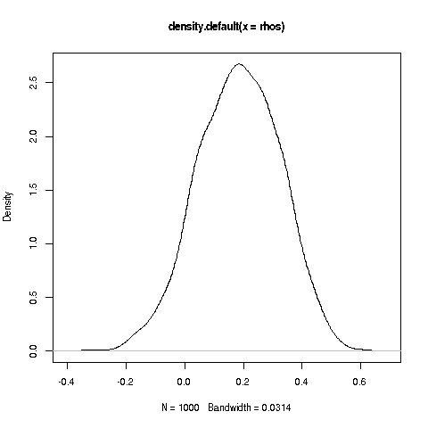
What do we see? The density is centered around 0.2, all right, but in some samples the estimated correlation is way, way higher, more than 0.6. Of course, the latter is an "accident," but if I look at many, many correlations (of different pairs of variables), "accidents will happen." This is the essence of p-hacking: Look at many quantities, finally finding one that one likes, and seizing upon it as a great "discovery" -- when it may in fact just be an accident.
Thursday, February 3, 1810The House Votes dataset will not be on tomorrow's quiz.
Thursday, February 3, 1640Tomorrow I will lecture on supplementary material on model selections. It is available here, in the inst directory for qeML in my GitHub repo.
Thursday, February 3, 1615For homework and exams, it will be assumed that you obtain the House Votes dataset via
download.file('https://archive.ics.uci.edu/ml/machine-learning-databases/voting-records/house-votes-84.data','hv.data')
Thursday, February 3, 0925
Two (unrelated) items:
Following up on my post of Tuesday, February 1, 1015:
The fact that R does not have call-by-reference is not a "deficiency" but actually a design philosophy. R is a functional language--again, all operations are functions, even '+' and '['--and the philosophy of functional languages is "no side effects." A function should not change the objects it works on. Thus the need to reassign the changed object after the call.
Since Q is less than full rank, then some linear combination of its columns is 0. (Or rows; remember, the row rank = the column rank.) So, Qw = 0 for some nonzero vector w. (This uses our material on partitioned matrices.) If Q were invertible, we could premultiply by its inverse, which would give us w = 0, a contradiction.
A student asked me what qeLin() is so slow on the InstEval data. Run
z <- factorsToDummies(ivl,omitLast=T)
dim(z)
to see why.
Wednesday, February 2, 1130If your group did successfully complete the original Problem 1, please contact me for an appointment for grading for Extra Credit. It will work just like the interactive grading, so I will ask each of you questions about what you did. That means each member of the group needs to be able to talk cogently about your work.
Tuesday, February 1, 2135In my 1900 post this evening, I wrote 'preds'; it should be 'holdoutPreds', fixed now.
Tuesday, February 1, 2110Concerning the Extra Credit offer for successfully completing the original Problem 1, the offer is still open now, provided you finish and turn in your code to me by the Monday deadline for Hwk 2.
Tuesday, February 1, 1900The revised version of Problem 1 is now on our Web page, with a full test case. You should find it easy to convert whatever previous work you'd done on the original Problem 1 to this new version.
Tuesday, February 1, 1015This post is devoted to the issues that arose in the original Problem 1. Even though that problem has been shifted to Extra Credit, it's important that you know what led to that.
Function arguments in R are treated as local variables, with a Copy on Write policy. For instance:
function(x)
{
   y <- x + 3  # line 1
   x <- y^2  # line 2
   return(x)  # line 3
}

w <- 5
f(w)
In the execution of line 1, x is still physically in the same memory location as w, but treated as a local variable in line 2; here w will be copied to a separate location, and references to x will be to that location.
Thus w will not change in the above code. As you know, if we want such a change, we need to have
w <- f(w)
But this was infeasible in Problem 1. This is why some groups found that changes to Aij from within a function were not being propagated outside the function. (One group did inform me of that, but then they said they fixed it, so I unfortunately just didn't give it further thought.) So, what are the solutions?
The best solution is to overload not only the read version of '[' but also the write, e.g.:
> d <- list()
>  d$v <- c(5,12,13,1)
>  class(d) <- 'abc'
> d
$v
[1]  5 12 13  1

attr(,"class")
[1] "abc"
>  `[<-.abc` <- function(obj,i,value) {obj$v[i] <- value; return(obj)}
> d[2]
[1] 12
> d[2] <- 88
> d[2]
[1] 88
Remember, in Object Oriented Programming terminology, the ability to overload operations like this is called polymorphism. Actually, even within R itself (as opposed to our "home grown" class above), the left bracket operator is subject to lots of overloading:
 methods(`[`)
 [1] [.abc                    [.acf*                   [.AsIs
 [4] [.bibentry*              [.check_details_changes* [.data.frame
 [7] [.Date                   [.difftime               [.Dlist
[10] [.DLLInfoList            [.factor                 [.formula*
[13] [.getAnywhere*           [.hexmode                [.listof
[16] [.news_db*               [,nonStructure-method    [.noquote
[19] [.numeric_version        [.octmode                [.person*
[22] [.POSIXct                [.POSIXlt                [.raster*
[25] [.roman*                 [.simple.list            [.table
[28] [.terms*                 [.ts*                    [.tskernel*
[31] [.warnings
To be continued.
Tuesday, February 1, 0955Reminders re using OMSI on quizzes:
Happy Chinese New Year to all! You don't have to be Chinese to enjoy this fun holiday.
Monday, January 31, 2130I'm embarrassed to say I messed up in Problem 1; it's just too hard. This evening I had various ways to make it easier, but each of the ways required that I have you learn very advanced aspects of R. From a programming language point of view, these are interesting, but they would distract from the main aspects of the course.
Thus I will delete the current version of Problem 1, and replace it with a similar but far easier problem. I'll do that tomorrow; too many other tasks need my attention this evening.
Very sorry for the inconvenience. If you have already finished Problem 1 in its original form, please see me about getting major Extra Credit.
As mentioned, I will move the due date back, to February 7.
It is important, though, that you understand the issues involved in the original version of the problem, which I will present in the next blog post.
Monday, January 31, 2005Several items.
Problem 1 specifies the 100K MovieLens version, but that is meant in contrast to the larger version, which has 27 million ratings rather than 100,000. It does not mean you use the ml100 data, for instance; use ml100kpluscovs, which has the side information.
A couple of days ago, a claimed in error in Problem 1. I was just about to look into it when the student wrote again, saying something like, "No, it was our misunderstanding," so I didn't take action. But another student brought it up today, and it was a valid concern.
I'll fix the wording in the homework this evening, but for now, a preview is that I want you to have the 'ratingsCache' objects in R environments. The latter are ways to achieve the conveniene of global variables without what some consider the "dangers." Again, details this evening, but for now, here is how R environments work:
> z <- new.env()
> z$a <- 3
> z$a
[1] 3
> z$a <- 8
> z$a
[1] 8
> f <- function(e,val) {e$a <- val}
> f(z,2)
> z$a
[1] 2
There are also ways to override assignment operators, but I want you to use environments, and important thing to learn.
Monday, January 31, 0030An alert student noticed that Aij in Problem 1 should be indexed by a character string, not a number. Thanks! I've changed the wording accordingly, and added clarification elsewhere in the problem.
Monday, January 31, 0020It's noted in the textbook in the mlb example, some columns have been deleted (Name, Team). If you try to reproduce the examples, keep this in mind.
Sunday, January 30, 2250Hi, everyone. I've gotten several inquiries about Problem 1 of Quiz 2, from students who mentioned the Central Limit Theorem but did not relate it to human height. But that relation was the core of the question. As I've emphasized, this is a course on math modeling, and the problem specifically asked about human heights.
Sunday, January 30, 0915Due to a 10:30 meeting, I will have to cut my 10 a.m. office hour short tomorrow. If there are further questions after that, please e-mail me. BTW, remember that the OHs will be in-person starting tomorrow, MW 10-11.
Saturday, January 29, 2115I've finished grading Quiz 2. (Stefan grades the homework, I grade the quizzes and term project.) The solutions are on our Web page. I had predicted there would be a couple of scores of 100; there was one, and a couple of 95s. Unfortunately, there were also a couples of 0s and 5s. Feel free to contact me if you have any questions.
Wednesday, January 27, 1940Important information the homework:
source('Problem1.R')
source('Problem2.R')
That will produce output! He will judge the technical correctness of your submission almost exclusively on the quality of your output, though he will also glance at your code.
I'm sure Stefan would appreciate it if you would insert statements like
print('output of test case on the conversion of the House Voting edataset:')
and
print('press Enter when ready')
In the case of Problem 2, his script will also open your .pdf file (which MUST be generated from .tex). He will read your analysis there; since this is an open-ended problem, it is imperative that your analysis be clear, cogent and professional.
In the latter, your group members must all present. (Once we switch to in-person instruction, this means PHYSICALLY present.) However, you are not graded as a group; EACH MEMBER RECEIVES AN INDIVIDUAL GRADE.
The technical correctness of the submission is taken as a given, and if so, a student's grade (not "the students' grade") starts at an A. But if the student then answers Stefan's interactive questions poorly, his/her grade goes down rapidly.
As noted in the syllabus, Stefan's questions will be things like "What does this part of the code do?" and "How would it change if the homework problem specs had instead been such-and-such?" He will also ask you general questions about the course material, e.g. "Why is a holdout set needed?" Of course, he will ask different questions to different students, both within and across groups.
Again: This is not a programming course! We do programming, yes, and you have to know the details, but the purpose of the programming is to support thought and usage of the mathematical concepts. As I stated at the beginning of the course, my goal is that at the end of the course, you will be able to apply the concepts of machine learning in general and recommender systems in particular, creatively and productively; my goal is NOT that you memorize the syntax of R, lm() etc.
Continuing my last post, about why CS students (or students from other majors who know computer systems well) have the background to go deeper into problem-solving:
A few minutes ago, I tried to install a package from CRAN, ClustImpute. I got an error message saying that my version of GSL was not new enough.
I investigated, and found that GSL is a C library. It is called by the R package of the same name but lower-case (which serves as a wrapper to the C), which in turn is called by the R copula package, which in turn is called by the R ClustImpute package. I did seem to have GSL on my machine (Linux in this case), and the test case seemed OK.
I downloaded the R source for gsl from CRAN, and found a configure file. Some of you may have heard of this, but I think most have not, and it's important to your status as a computer expert, so let me explain.
A configure script is part of autoconf, a system of Unix shell scripts that are used to build a library. They are typically used on C/C++ code, and that is the case for the C library GSL.
In other words, when I tried to install the R package gsl, it ran the configure script to check my machine's environment. That script gave me the error message.
So I open the script in Vim and searched for the message. After finding it, I looked at the lines above, and found that it has failed to open the directory /usr/local/include/gsl on my machine. I checked, and it turned out to be non-world-readable. I fixed that with chmod, and then everything installed fine.
Nothing deep here, of course. But it shows how valuable CS "street smarts" can be.
Wednesday, January 27, 1135You will be using my regtools, rectools and qeML packages (and later, some packages others have written). If an R package is on the CRAN repository, one can use install.packages() to do so. However, the regtools version on CRAN is not up to date, and the other two are not on CRAN yet. You must install them from my GitHub repo.
R expects you to store installed packages in one or more directories that you specify. If you are using RStudio, it probably has already set one up for you. If not, you can specify them in your ~/.Rprofile startup file; in mine, I have lines like
.libPaths("/Users/normanmatloff/R")
I store my installed packages in ~/R, and this line says R should look there whenever I call library() to load a package.
To download qeML, for example, you can install devtools (you may already have it), then load it and type
install_github('matloff/qeML')
Personally, I'd rather do things on my own. I would type in the shell (not R)
git clone http://github.com/matloff/qeML
R CMD INSTALL -l ~/R qeML
I do this because I often want to look at the code in the downloaded package.
BTW, I don't use RStudio. It's wonderful for non-techies, but IMO it gets in the way in the case of R "power users." Actually, there are R IDEs more suited for CS people, notably the Lisp-based ESS (Emacs Speaks Statistics), but for me, I prefer direct interaction with R. I use the Vim editor (for everything, not just R), with my own home-grown macros and abbreviations.
Wednesday, January 27, 1035Note that the predict() functions work on multiple new X values. For instance, on p. 50, we might have
predict(lmout,data.frame(Height=c(73,71),Age=c(25,28)))
I've added a section on the LASSO in the text, and you may use it in Problem 2 if you wish.
Wednesday, January 27, 0715Starting with Quiz 2, you'll need the following on your computers:
Tuesday, January 25, 1515Note: In matrix contexts, R treats vectors as rows or columns rather flexibly. If one uses a vector in a matrix context, R will try to guess what we mean.
> u <- 1:3; v <- c(5,1,8)
> u %*% v  # no need for t()
     [,1]
[1,]   31
> t(u) %*% v  # OK too
     [,1]
[1,]   31
# but if a matrix and not a vector, rows and columns matter
> u <- matrix(u,nrow=1)
> u %*% v
     [,1]
[1,]   31
> u <- matrix(u,ncol=1)
> u %*% v  # v is taken to be a row!
     [,1] [,2] [,3]
[1,]    5    1    8
[2,]   10    2   16
[3,]   15    3   24
Best to convert vectors to 1-row or 1-column matrices to be sure.
Tuesday, January 25, 1240There are only two problems in Hwk 2. But definitely enough to keep you busy. :-)
In Problem 1, "Don't miss the forest for the trees!" I've added this to the specs, just to make absolutely sure no one misses the point:
Remember, the point is to give the illusion that we are actually accessing the matrix in memory!
Note that I have also added a constructor.
Monday, January 24, 2130Hwk 2 is ready!
It is due Feb. 3, which sounds like a long time from now, but there is quite a bit to do. And, if one of your team members is returning from abroad, that may cause complications.
START EARLY! You have enough background now to do Problem 1, and will have most of the needed background for Problem 2 after Wednesday's lecture (you may wish to read ahead).
If the TA feels that one or more groups has done an especially good job on Problem 2, he will award Extra Credit.
Monday, January 24, 1835As you can see from today's lecture, linear algebra will be more and more important as the course progresses. I recommend that you do a quick review of the linear algebra chapter, and also become adept at using R in that realm, especially %*% and solve().
Monday, January 24, 1525I am assigning as a supplement to our textbook my stat/R blog post on double descent. This is one of the most interesting developments in the stat/ML area in the last few years, potentially turning upside down some cherished views.
You'll need to know about polynomial models to understand this post. I'm not sure we'll get to this on Wednesday, but you can read ahead or wait until Friday.
Monday, January 24, 1135I've added the questions file for Quiz 1 to our directory.
Monday, January 24, 0820I've placed the Quiz 1 solutions on our Web page. Please note:
Quiz 1 grades are being mailed out as I write this. I have the following remarks:
I will post solutions tomorrow.
Sunday, January 23, 2115Regarding the issue of carefully following directions:
After Quiz 1, Stefan told me a few students had trouble with the load(Hwk1.RData) line. They had to seek help from Stefan, wasting precious minutes of quiz work time. And worse, some DIDN'T seek help from Stefan, and wrongly assumed that a directory ml-100k/ would be present. Of course, that meant their code would have no chance of working.
I didn't realize what was going on in this regard until I was halfway through grading the quiz. So it was too late for me to add the directory and then start grading all over again, even if that were justified, which is debatable.
One student had a comment line in the solution to one of the coding problems in the quiz:
# why can't we have an ml-100k/ directory, like on the homework?
The answer is that the homework did NOT have such a directory. The specs said that only Hwk1.RData would be present. And the blog said that the environment in the quiz would be the same.
Presumably the Hwk1 submission for that student's group likewise made use of a ml-100k/ directory, and WILL BLOW UP WHEN STEFAN RUNS HIS GRADING SCRIPT. If your code was like that, send Stefan e-mail immediately, so that he can go ahead and set up such a directory before he starts grading. By this post, I'll have Stefan impose no penalty this time.
Simon Says is for preschoolers.
Sunday, January 23, 1955I am still not done grading Quiz 1. I'm working on getting Hwk 2 out, to make sure you have plenty of time to do it.
Wednesday, January 19, 1110A student mentioned getting an error message from density(), stating that the vector given to it was too short for bandwidth computation. That would mean that one of the genres consisted of any a single movie. I'm surprised to hear this, but if it's true, just omit that genre in your test of plotDensities().
For Extra Credit, though, add some exception handling code, using R's try() or tryCatch() function, to gracefully handle such situations. The code will skip that particular factor level, and call warning() wtih an appropriate message stating the level.
Wednesday, January 19, 1100The general instructions for submitting homework mention .tex files. These are for textual material, e.g. commentary on code output. We don't have any for Homework 1.
Wednesday, January 19, 09501. You are all computer experts. 2. Grading administration in our class is done by computer. 3. Therefore, you know that all procedures (homework, quizzes, project) must be done EXACTLY ACCORDING TO SPECIFICATIONS.
In particular, all of your records in the class are indexed by your official UCD e-mail address (the one I use to mail you). So, if you submit a quiz, say, using your personal GMail address, your grade will be invisible when I make course grades at the end of the quarter.
Of course, I do have some protections against such a calamity in my scripts, but nothing is perfect. Make sure to follow the specs EXACTLY.
Tuesday, January 18, 1940Another handy trick, similar to that of the blog post of January 18, 1045: A handy way to get counts.
> x <- c(1,5,8,2,3,12,3)
> sum(x == 3)
[1] 2
> sum(x < 8)
[1] 5
Tuesday, January 18, 1755
Our first "real" quiz will be held this Friday. Note the following:
The "official" version of Chapter 3 is now ready. It would suggest obtaining now, because tomorrow morning there will be a rebooting of the department server that hosts faculty Web pages. For that matter, this blog is there too, so be sure to keep up to date. When a server is rebooted, one never knows what may happen.
Tuesday, January 18, 1045Here is a handy R trick to keep in mind. Say you want to find the proportion of values in a vector x that satisfy some boolean condition. You can use the fact that the mean of a set of 0s and 1s is the proportion of 1s.
> x <- c(8,5,12,13,3,4,5)
> mean(x == 5)
[1] 0.2857143
> mean(x >= 8)
[1] 0.4285714
Monday, January 17, 0815
Happy MLK Day! It's a holiday, so I normally would not hold my Monday office hour, but I could easily do so if there is any interest. If you would like to meet with me during 10-11, send me an e-mail message and I will be there (virtually).
Sunday, January 16, 2300A note on object-oriented programming with R:
R gives one various choices regarding OOP. The most commonly-used is S3, and there are also S4 and R6. Each one of those has its fans.
S3 implements the general programming language principles of encapsulation and polymorphism. Let's see how these work in the case of the function density().
An S3 object is actually an R list, with the components of the object being the components of that list. In the previous blog post, we mentioned the $y component, which is the vector of y-coordinates of the curve to be plotted. Let's see what else is in there, using the R built-in dataset Nile:
> q <- density(Nile)
> str(q)
List of 7
 $ x        : num [1:512] 274 277 279 282 284 ...
 $ y        : num [1:512] 7.40e-07 8.34e-07 9.43e-07 1.06e-06 1.19e-06
...
 $ bw       : num 60.6
 $ n        : int 100
 $ call     : language density.default(x = Nile)
 $ data.name: chr "Nile"
 $ has.na   : logi FALSE
 - attr(*, "class")= chr "density"
You can see the x-coordinates there, and various other things. The bw component is the bandwidth, which is analogous to the bin width in a histogram. Note that the class of the object is 'density'.
So all those things are "encapsulated" into one handy package. What about polymorphism? It means that functions have different actions, depending on the class of object they are called on.
Let's print. In interactive mode, we can print just by typing the expression, without having to explicitly call print()
> q

Call:
        density.default(x = Nile)

Data: Nile (100 obs.);  Bandwidth 'bw' = 60.63

       x                y
 Min.   : 274.1   Min.   :7.397e-07
 1st Qu.: 593.5   1st Qu.:5.624e-05
 Median : 913.0   Median :4.486e-04
 Mean   : 913.0   Mean   :7.818e-04
 3rd Qu.:1232.5   3rd Qu.:1.397e-03
 Max.   :1551.9   Max.   :2.380e-03
You might have expected $x and $y to be printed. But instead, here is what happens:
The R function print() is known as a generic function, meaning it's just a placeholder. Our call print(q) is dispatched according to the class of q, which is 'density'. Thus our call is relayed to print.density(q), i.e. a print function that the developers of R wrote specifically for that class. Whoever wrote that function decided that the output we see above was best.
Another generic function in R is plot(). So, plot(q) will be dispatched to plot.density(q).
You can think of R generic functions in terms of function override, as in C++.
The ggplot2 package overrides '+'. The latter actually IS a function:
> 2+5
[1] 7
> '+'(2,5)
[1] 7
Let's see how to do the equivalent of hist(Nile) in ggplot2:
> w <- ggplot(data=pef)
> ww <- w + geom_histogram(aes(x=wageinc))
> ww
Again, ggplot2 overrides '+', with the "sum" being a new graphics object. Here w was just an empty graph, and we "added" a histogram to it, making a new object that we assigned to ww.
We then "printed" ww to display the graph.
You as a user can write your own S3 classes. You simply create an R list with the components you want, and give it a class name, eg.
> str(u)
List of 2
 $ a: num 3
 $ b: num 8
 - attr(*, "class")= chr "myclass"
Optionally, you can add some generic functions. Sunday, January 16, 2240
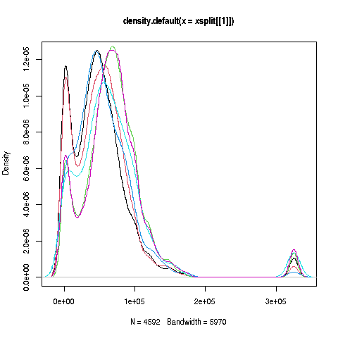
plotDensities(pef,'wageinc','occ')
There are 6 occupations in this dataset.
In both graphs, we are plotting wage income. Type '?pef' to learn more about the dataset.
Of course, the function plotDensities() here is rough. It took me about 1 minute to write (but 7-8 minutes to debug!), just doing what is suggested in the homework specs, with calls to split(), density(), plot() and lines(). It needs to make better labels (giving the user options for this too), and display a legend, so we know which curve is which.
Also, look at the graph-by-gender. The red curve is literally "off the charts." To remedy this, plotDensities()would need to look at the return values from the calls to density(). The latter function returns an object of class 'density', the $y component of which is a vector showing the y-coordinates of the points on the curve (512 points by default). Our function could then determine which curve is highest, and then plot that one first.
With graphics, one should know a number of packages, then use the one best suited to the application at hand. For instance, ggplot2 automatically handles the "off the charts" problem, and automatically provides legends. And there are many graphics specialty packages that are built on top of it. But it is less flexible than base-R graphics, and is not well-documented. The lattice package is also quite nice.
Sunday, January 16, 2040Rough example. Will comment more later.
library(regtools)
data(pef)
plotDensities(pef,'wageinc','sex')
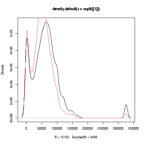 Sunday, January 16, 1900
I made a mistake, very sorry! In this blog post, I'm going to explain what the mistake was, how it was fixed--and why you should have caught it. (At least, the ones who've already begun work on Problem 3 should have caught it.) I'm not trying to make excuses for myself--a mistake is a mistake--but I do want to make a learning opportunity out of this. (BTW, I've moved the due date back to Thursday.)
The error was simple but crucial: I neglected to state what "X" is: Mean rating. See the revised problems specs for details.
Now, how should you have known that? Why not plot ratings, rather than mean ratings? The answer is in the prerequisite review (ECS 132, STA 131A or similar) at the beginning of the problem specs: A density is for a continuous random variable. Some people took X to be movie rating, but that is discrete, integer valued, not continuous.
The point then is, without knowing what X is, those who've started on Problem 3 should have asked.
This is important. A homework bug is just like a program coding bug, or for that matter, a typo in a report: One can check it a mlllion times, but the more one checks, the more likely it is that one catches the error. I had Stefan check it too, of course, but he didn't catch it either.
In summary:
Say for example there are just two users. The function will input the two timestamps vectors, and will output the vector of sorted, merged timestamps. The merging comes from comparing the current element of input 1 with the current element of input 2; whichever is smaller goes into the output, and the current pointer for that input is advanced by 1 element.
That has time complexity O(n). What you should NOT do is concatenate the 2 inputs and then call sort(); that has complexity O(n log n). Which is better?
In Problem 1, the first wait time is from the first timestamp to the second. (I've changed my post of January 15, 1545 accordingly.)
Saturday, January 15, 2145Columns G1-G19 are dummy variables individually, but not collectively, i.e. they do not collectively code a categorical variable. This is because a given movie can have more than one genre.
Recall that the (revised) homework specs say, "If in any row there are multiple genres, choose one at random, by calling sample()." That implies that you will set the other 1s in that row to 0s.
Saturday, January 15, 1620I forgot to write "the mean of" in my last post, corrected now.
Saturday, January 15, 1545Please make sure you've read my 1325 post (if you are among the 2 or 3).
Now concerning Problem 1:
W is the mean of the set of times between events from any user. Let's say that each user rings a bell each time they post a rating. Then W1 is the mean of the times between bell rings by user 1. W2 is the mean of the times between bell rings by user 2. W is the mean of the times between bell rings of any source.
Say user 1 has timestamps 1.2, 5.9, 6.1 and 7.0, and user 2 has timestamps 2.2, 4.4 and 8.8. W1 is the mean of 4.7, 0.2, 0.9. W2 is the mean of 2.2, 4.4. W is the mean of 1.0, 2.2, 1.5, 0.2, 0.9, 1.8. E.g. W = 1.257.
Saturday, January 15, 1325After Stefan had people use the campus VPN, I believe there were only 2 or 3 who were not able to submit yesterday's quiz. Those 2 or 3 will get a second chance next Tuesday, when Stefan will have an OMSI server open throughout the say, 10 a.m. to 10 p.m. He will announce the machine and port by e-mail.
Note that Stefan will have an office hour that day, in which he can help anyone who is having trouble with OMSI.
Again: Note carefully that we will have quizzes every week, and that they count 70% of your course grade.
Friday, January 14, 2245What Can Go Wrong with Computers, Part III:
Last but not least: Why couldn't I share my Zoom screen in the last two lectures?
When I tried to share, Zoom told me to go to the Security and Privacy tab, to allow Zoom to access my screen. When I got there, the Zoom icon was a faint gray. I clicked the icon, and it turned bright blue. I unlocked the lock etc. But I still couldn't share my screen. Zoom ketp sending me back to the Security and Privacy tab.
The Web was no help. I rebooted, no help. I reinstalled Zoom, no help. I reinstalled Zoom on the M1 emulator, no help.
But then...I noticed something I hadn't seen before. Next to the Zoom icon, which had changed from faint gray to bright blue, there was a faint gray box! I was supposed to check it! I did, and now can share my screen.
I am mainly a Linux user, but do have several Macs, which I prefer for Zoom. Maybe if I were more accustomed to the Mac UI, or had better computer-distance eyesight, I would have noticed the faint gray box earlier.
"All's well that ends well."
Friday, January 14, 2115What Can Go Wrong with Computers, Part II:
As I said, your quizzes form 70% of your course grade, so it is crucial that you master OMSI. Note the following:
Whenever accessing a campus entity, you should make sure to use a campus VPN. I think you all know about the one in the library. There is also one run by the College of Engineering, which I use, but after reviewing the e-mail sent by administrators when this started, apparently it is not open to undergrad students.
In order to have Quiz 1 go smoothly, do a test (well before next Friday, in case anything goes wrong) in which in you run the OMSI server on a CSIF machine, and the OMSI client on your own machine at home. Note that the default Python version on CSIF is 2.7, so make sure to run python3 rather than python.
Please interact with Stefan (well before next Friday), if you encounter trouble.
Friday, January 14, 2100What Can Go Wrong with Computers, Part I:
With Stefan's permission, I'm posting his comments on difficulties with the genre data. As he says, only a handful of cases is affected, so don't worry about it. But I do want you to learn from it. This is how data is in the real world -- messy!
From: Stefan Broecker
********************************************************
Hi Dr. Matloff,
A student during office hours brought up an issue they saw in the data produced by the r script you provided them They noticed that a few of the movies were showing up in the data with NA genres, and noticed that they corresponded to movies in u.item with special characters in their names (Les Misérables for example).
I then went through the script to see if I could figure out what was going wrong and I think I found the culprit and a solution. It looks like on this line:
zs <- strsplit(z,'|',fixed=3DTRUE) # splits to single characters
strsplit is throwing an error because of an "invalid locale." I was able to get the script to work by adding the flag useBytes=TRUE. So:
zs <- strsplit(z,'|',fixed=3DTRUE,useBytes=3DTRUE) # splits to single characters
With the added flag I don't see any movies in the data with NA for a genre.
The issue only affects 5 movies as far as I can tell so it's not a huge deal, but I still thought you'd want to know about it.
Best, Stefan
********************************************************
By the way, "locale" in the R context means language, e.g. English or Spanish, or for that matter, American English vs. British.
Friday, January 14, 1245A few people had trouble with OMSI this morning, according to Stefan. As you know, the quizzes are 70% of your grade, so it is imperative that you remedy this NOW.
First, if you were in that situation, send me the following information, cc-ing Stefan:
Please get this information to Stefan and me IMMEDIATELY
Thursday, January 13, 2240The wording in Problem 1 concerning output was a bit unclear, so I've elaborated on it.
Feel free to contact me if you are unsure about anything in the assignment.
Thursday, January 13, 2150Please make sure you completely understand the process that Stefan will use to check your homework submissions.
He will run a script, like the outline I showed in the homework specs. Other than execution errors or infinite loops -- which of course WILL NOT HAPPEN, RIGHT? :-) -- the process will be automated.
Stefan will mainly look at your code's output when he runs it via his script. He'll glance at your code too, but mainly he'll look for the proper output, both printed (ie stdout) and graphical.
As you see in the script, it will call source('Problem1.R' etc. So, YOU should be able to do the same. If you make that call, say from the '>' prompt, and you don't get the proper output, then your code will similarly fail when he makes the same call. MAKE SURE TO AVOID THIS.
It would be very beneficial if you were to look at the script outline in detail, both to learn more R and also to imagine how things will play out when Stefan checks your code.
Wednesday, January 12, 1140Recall that I am basically writing our textbook as we go along. Much of the material is there, but much needs to be filled in. Accordingly, the full book file will constantly change, but the early parts will be "frozen." I'll make separate files that, while containing the full book, will not change in the indicated chapters. Their names will contain the term "Official."
So, the file Ch1Official.pdf , that I've had up there for a while now, will contain the final, frozen version of Chapter 1.
I've now done the same for Chapter 2, in the file Ch2Official.pdf . It also contains the official Chapter 1.
Wednesday, January 12, 1140This example may help your thinking in Problem 3:
tg <- ToothGrowth
plot(tg$len)
plot(tg$len,col=tg$supp)
Run this yourself! Just copy-and-paste from the above.
What happened here? First, I created an abbreviation, 'tg', to avoid lengthy typing. (I also could have used the R with() function.) Here ToothGrowth is one of the built-in datasets in R. Then I plotted the tooth length, without regard to what supplement was used. Then I plotted again, this time color-coding the supplement.
What happened internally? The plot() function looked at its col argument, and split the data according to that factor. It then plotted each of the resulting groups in separate colors.
Your function in Problem 3 will follow a similar pattern. Its grpName argument will be analogous to col. It will split the data--i.e. the column in inputDF designated by xName--into groups according to grpName, then draw a density estimate for each one.
As noted in the blog post of January 6, 1535 and as emphasized in class, your plotDensities() function must be GENERAL. Its code must not be tied to MovieLens, recommender systems etc.
But you will call plotDensities() on ml100kpluscovs, and in order to do so, you'll need to add an extra column to that data frame, say named 'genre'. It will be an R factor, consisting of numbers, ranging from 1 to 19. (If in any row there are multiple genres, choose one at random, by calling sample().) You'll need to convert the genre dummy columns to this. I suggest that you make use of a function in the regtools package; I don't have it in front of me as a write this, but install and load that package (from my GitHub repo, 'matloff'), and run
ls(package:regtools)
and you'll see it.
Wednesday, January 12, 1125Mystery solved! (I think.) During lecture today, I could not share my screen. The windows weren't even listed right. Fortunately, Stefan was present and saved the day by sharing his screen.
But what caused the problem? Well, after class and my OH, I got a message, "New version of Zoom successfully downloaded." Apparently a new version was downloading DURING my usage. I don't recall whether I requested it, but I think this was the cause. No wonder it asked me to set permissions when I tried to share my screen.
Tuesday, January 11, 2330The R function unique() is very handy. Make sure you know how to use it.
Monday, January 10, 2140A riddle on Twitter asks what the R value of (1:3)^NA is. I have to admit that my guess was wrong. Behold:
> (1:3)^NA
[1]  1 NA NA
After all, 1 to any power is 1, even if the power is unknown.
Monday, January 10, 1950As noted, due to my late start to my office hour today, I am planning to set up a special hour sometime. I'm considering Wednesday or Thursday evening of this week. If you believe you'd likely partake of such an hour please let me know by e-mail.
Monday, January 10, 1910A student has set up a Discord group for our class. As I explained, I am not a fan of Discord, Piazza, etc., a least not for a course requiring deep intuition such as our. You are of course welcome to join the group, but please note I will not be monitoring it; if you have a question, please e-mail it to me or bring it up in my office hour.
Monday, January 10, 1700OK, ready to go. I've added an adjacent file Diff.html, the output of running diff on the old and new versions.
Monday, January 10, 1640After reading a student query, I see there are some ambiguities in Hwk 1. I'm fixing them now, will announce when I'm done (a few minutes, I think).
Monday, January 10, 1105Apologies again for my messing up. To compensate, I'll set an extra office hour, probably in the evening, maybe tomorrow evening. Watch this space.
Monday, January 10, 10:30Looks like I got confused re OHs. I thought I'd set them at 11, not 10. But I'm here now in the Zoom room, will be here until 11.
Sunday, January 9, 2235Homework teams are set! List is here.
Friday, January 7, 2110Now that the university has gone virtual until February 28, I've changed my hours to Zoom, via Canvas. Same days/time, MW 10-11. If the university goes back to in-person after 2/28, then I will too.
Friday, January 7, 10:25Sorry, had to cancel class. Could not connect using my laptop, for some reason. Switched to desktop, but had host issues, not sure why.
Friday, January 7, 10:00I am trying to connect to the campus link from home, no luck yet. Please be patient.
Thursday, January 6, 2300Just in case there was any confusion: We WILL have discussion section tomorrow. Stefan will lecture on R, especially aspects that will be very important in our course. Remember, discussions will always be at 9 a.m. Fridays, in 168 Hoagland, and Friday lectures will be at 10, in 212 Wellman. Of course, the room numbers will be irrelevant through 1/28.
Thursday, January 6, 18:35Problem 3 is now complete. I made a couple of very minor changes for clarification in Problems 1 and 2, so please take another look at them. After Stefan gives me the OK, I'll announce that one ready too, but it's certainly ready for you to start now.
Thursday, January 6, 1535Please note that, unless stated otherwise, when a homework prompt says "Write a function with call form...," it means literally that, GENERAL. Do NOT tailor it to the dataset or application in the homework problem.
Re error checking: We will not require it, but for your own pride of work, I would suggest including it.
Thursday, January 6, 14:40To clarify: Quiz 0, on OMSI, will be held on January 14. Quiz 1, the first "real" one, will be on January 21. (But Quiz 0 definitely counts in the course grade like another quiz.)
Thursday, January 6, 13:00Cloud recordings of lectures now up to date, sorry for the delay.
Thursday, January 6, 10:10Please read--in detail-- this R script, which you will use to generate the dataset ml100kpluscovs, which is used in our book and will be used in the present homework. In addiition to the use of the dataset, there are lots of important R constructs there. Let Stefan or me know if you have any questions.
Wednesday, January 5, 2310Problem 2 is now ready!
Wednesday, January 5, 2155Problem 1 in our homework is ready! There might be a couple of small tweaks after Stefan looks it over, but it's basically ready. Problems 2 and 3 in progress.
Wednesday, January 5, 1715I've already started writing the homework specs, here. So far I just have the ground rules, but you can get an idea of what will be involved from that, and the problems themselves should be out by Friday at the latest.
Wednesday, January 5, 1525Again, note the availability of the old quizzes and solutions here. Keep in mind:
On Friday, January 7 in discussion section, we will have Quiz 0, whose sole purpose is to make sure you know how to use the OMSI exam software.
Everyone "should" get an A+ on the quiz. Here are the actual grades from my ECS 132 class last year:
> z <- read.table('qg',header=F)
> table(z[,7])

A+  B B+  C  D  F
81  1  3  2  1  1
Draw your own conclusions. :-)
There will be two problems, one using R code and the other an extremely brief "essay" (text answer).
To do well on Quiz 0, and to insure being problem-free in the other quizzes:
Also, make sure to read the OMSI part of our syllabus again.
Tuesday, January 4, 09:25Two items:
As a student mentioned in class, our textbook is here
One thing you may wish to do is browse through the mathematical content of the book, especially Chapters 2, 5 and 6. Those chapters are not quite ready yet, but they should be enough to inform you as to the mathematical level of the course.
As noted, as of now, only Chapter is "official," with the rest currently being worked on. Each time a chapter becomes official, I'll post a frozen version of it.
Monday, January 3, 1700Rooms, times, roles:
Whenever I say "lecture," I mean MW 9-10 Hoagland, F 10-11 Wellman; "discussion" means F 9-10, Hoagland.