Well, that's enough meaningless calculating for now. Let's do some data analysis!
R includes a few dozen small but real data sets built in, for demonstration purposes. You can see a list by typing "data()" at the prompt. But let's look at a specific one, named Nile:
> Nile
Time Series:
Start = 1871
End = 1970
Frequency = 1
  [1] 1120 1160  963 1210 1160 1160  813 1230 1370 1140  995  935 1110  994 1020
 [16]  960 1180  799  958 1140 1100 1210 1150 1250 1260 1220 1030 1100  774  840
 [31]  874  694  940  833  701  916  692 1020 1050  969  831  726  456  824  702
 [46] 1120 1100  832  764  821  768  845  864  862  698  845  744  796 1040  759
 [61]  781  865  845  944  984  897  822 1010  771  676  649  846  812  742  801
 [76] 1040  860  874  848  890  744  749  838 1050  918  986  797  923  975  815
 [91] 1020  906  901 1170  912  746  919  718  714  740
These are flow numbers of the Nile River. You can see there are several rows of data. How many numbers in alll? Well, it says this is for the years 1871-1970, so there should be 100 numbers, but how can we confirm it? We can start counting in the row labeled 91, so 906 is observation 92 and so on, and we see that the last number, 740, is the 100th. But the short way is to simply ask:
> length(Nile)
[1] 100
Here we are using the built-in R function length(). A function is simply something that take one or more inputs, and gives an output, in this case the length.
Note that Nile is an R vector, meaning simply a bunch of values on a certain variable, in this case river flow. We applied the length() function to that vector, producing the number 100, and recall from above that any numerical expression we type at the prompt will be printed out, as here.
Now suppose we want to know the number for the year 1899. That's the 29th year (not the 28th), so we need the 29th number, which we can get using brackets:
> Nile[29]
[1] 774
The number 29 here is an index. We can ask for ranges too, say indices 55-58:
> Nile[51:58]
[1] 768 845 864 862 698 845 744 796
The 51:58 means the numbers 51 through 58. Let's check it:
> 51:58
[1] 51 52 53 54 55 56 57 58
Using R's function c() ("concatenate"), we can request even noncontiguous indices, say request Nile elements 1, 98 and 100:
> Nile[c(1,98,100)]
[1] 1120  718  740
Note that in each case above, I am creating a new vector from an old one. For example, the expression Nile[c(1,98,100)] is a 3-element vector. If I will be using it a lot, I should give that new vector a name:
> y <- Nile[c(1,98,100)]
> y
[1] 1120  718  740
> length(y)
[1] 3
The '<-' is R's assignment operator. We say that we assign Nile[c(1,98,100)] to the variable y. I can subsequently assign something else to y if I wish:
> y <- 28
> y
[1] 28
R has excellent graphics capabilities. We will work with some elaborate ones later, but for now, let's stick to a plain-Jane one, a no-frills histogram:
> hist(Nile)
At this point, a window pops up on the screen:
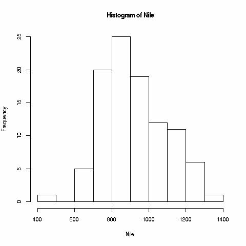
Again, this is not fancy yet, but it's a start.
We can do a time series plot too:
> plot(Nile)
Again a window pops up, and we get:
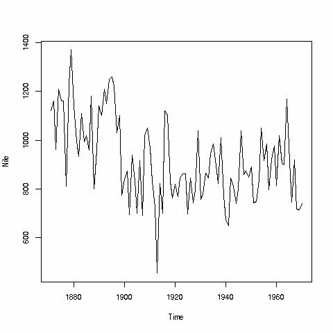
R is what is known as an object-oriented language. In this context, it means that we can use the plot() function on lots of different kinds of objects, and R will figure out what kind of plot is appropriate. Here we had time series data, so R plotted accordingly. If we had (X,Y) data, say people's heights and weights, R will draw a scatter plot, which we will do in a future lesson.
We can find means, e.g.
> uvw <- c(1,20,25)
> uvw
[1]  1 20 25
> mean(uvw)
[1] 15.33333
Another useful function is which(). Say we want to find in which years the flow was greater than 1000:
> which(Nile > 1000)
[1]  1  2  4  5  6  8  9 10 13 15 17 20 21 22 23 24 25 26 27 28 38 39 46 47 59
[26] 68 76 84 91 94
For instance, this says that the 5th data point was larger than 1000. Let's check it:
> Nile[5]
[1] 1160
Again, here 5 is known as the index (or subscript) we are using to specify vector element(s).
Say we want to determine in which years the flow was more than 1000. Well, remember, index 1 is for year 1871, index 2 is for year 1872 and so on. So, all we have to do is add 1870 to each of the indices above:
> which(Nile > 1000) + 1870
[1] 1871 1872 1874 1875 1876 1878 1879 1880 1883 1885 1887 1890 1891 1892 1893
[16] 1894 1895 1896 1897 1898 1908 1909 1916 1917 1929 1938 1946 1954 1961 1964
There is a subtlety here that should be explained, though. To see it, let's re-do the above, saving the output of which() for clarity:
> q <- which(Nile > 1000)
> q
[1]  1  2  4  5  6  8  9 10 13 15 17 20 21 22 23 24 25 26 27 28 38 39 46 47 59
[26] 68 76 84 91 94
> q + 1870
[1] 1871 1872 1874 1875 1876 1878 1879 1880 1883 1885 1887 1890 1891 1892 1893
[16] 1894 1895 1896 1897 1898 1908 1909 1916 1917 1929 1938 1946 1954 1961 1964
Here q is a vector of length 30. By contrast, R regards the number 1870 as a vector of length 1, a mismatch of lengths. So, R recycles 1870 into a vector of 30 copies of the number 1870, and then adds that new vector to corresponding elements of q.
Actually, even in the expression Nile > 1000 above, the 1000 was recycled to a 100 copies of the number 1000.
Now, on to Lesson 3.