In Lesson 2, we learned about R vectors, a workhorse data type in R. Another workhorse is the data frame, which will be introduced in this lesson.
The concept is simple: A data frame is a collection of vectors. All of these vectors are describing different aspects of the same entities, e.g. the same people, the same countries, etc.
For instance, suppose we have height, weight and age data on 4 people. The would mean a height vector, length 4, and a weight vector, same length, and an age vector, again of length 4:
| height | weight | age |
| 64 | 135 | 42 |
| 72 | 181 | 33 |
| 68 | 132 | 52 |
| 61 | 135 | 76 |
So, each column is a certain variable, say age, and each row is for a certain person, such as the person who has height 64, weight 135 and is of age 42. Each column has a name, either provided by the person who creates the data frame, or default names V1, V2 and so on. We could have many more columns, e.g. birthdate, name and so on.
By the way, R does allow for missing values, coded NA for "Not Available," e.g.
| height | weight | age |
| 64 | 135 | 42 |
| 72 | 181 | NA |
| 68 | 132 | 52 |
| 61 | 135 | 76 |
That second person's age is unknown.
Let's look at a real data frame, again from R's built-in data sets, a list of which you can get by typing "data()". Let's try the airquality data frame,
We could print the entire data set to the screen, as usual by simply typing its name, but some data sets are too voluminous for this. Instead, let's use R's head() function:
> head(airquality)
  Ozone Solar.R Wind Temp Month Day
1    41     190  7.4   67     5   1
2    36     118  8.0   72     5   2
3    12     149 12.6   74     5   3
4    18     313 11.5   62     5   4
5    NA      NA 14.3   56     5   5
6    28      NA 14.9   66     5   6
The function has displayed the first six rows, i.e. the first six days, and we see various air quality variables. Their names are obvious, except for "Solar.R"; what's that?
To answer that question, we turn to R's online help facility, which we can invoke via a question mark (or another function, help()). So we type "?airquality",
> ?airquality
and the first few lines of output are
airquality              package:datasets               R Documentation

New York Air Quality Measurements

Description:

     Daily air quality measurements in New York, May to September 1973.

Usage:

     airquality

Format:

     A data frame with 154 observations on 6 variables.

       '[,1]'  'Ozone'    numeric  Ozone ()
       '[,2]'  'Solar.R'  numeric  Solar R (language)
       '[,3]'  'Wind'     numeric  Wind (mph)
       '[,4]'  'Temp'     numeric  Temperature (degrees F)
       '[,5]'  'Month'    numeric  Month (1-12)
       '[,6]'  'Day'      numeric  Day of month (1-31)

:
Note the colon in the last line above. It signifies a pause, so that we see the output only one screenful at a time, obviating the need for us to take a speed reading course! We can go to the next screenful by hitting the Space bar, or if we don't wish to read further, we hit the q key ("quit"). In the second screenful (not shown above), we learn that Solar.R is the amount of solar radiation.
R's online help facility is quite handy. Suppose for instance that we wish to learn more about the head() function. We type "?head", and discover that there's quite a bit more to this function:
head                   package:utils                   R Documentation

Return the First or Last Part of an Object

Description:

     Returns the first or last parts of a vector, matrix, table, data
     frame or function.  Since ‘head()’ and ‘tail()’ are generic
     functions, they may also have been extended to other classes.

Usage:

     head(x, ...)
     ## Default S3 method:
     head(x, n = 6L, ...)
     ## S3 method for class 'data.frame'
     head(x, n = 6L, ...)
     ## S3 method for class 'matrix'
     head(x, n = 6L, ...)
     ## S3 method for class 'ftable'
     head(x, n = 6L, ...)
     ## S3 method for class 'table'
     head(x, n = 6L, ...)
:
Among other things, we find that there are different forms of head(), corresponding to different object types. Our object type above was data frame, but for example if we used head() on an object of table type, head() would have behaved in a manner more suitable for that type.
Recall that this illustrates the object-oriented nature of R: The same function, in this case head(), may act somewhat differently for different types of objects.
Note the following part of the above output:
     ## S3 method for class 'data.frame'
     head(x, n = 6L, ...)
In our call
head(airquality)
we had provided to head() just one input, in programming parlance one argument (or, one parameter). But now we see that head() has a second argument, n. It is optional, a property signified by the equal sign. If we want the first 10 rows of our data frame, say, instead of 6, we can use the call
head(airquality,n=10)
Indices or subscripts in data frame take the form of pairs, a row number and a column number. Or, we can access the specified item by treating its column as a vector. For instance, to get the temperature on the 10th day, we have a couple of options:
> airquality[10,4]
[1] 69
> airquality$Temp[10]
[1] 69
In the first case, we used the fact that temperature is in column 4. We wanted row 10, for the 10th day, so we wrote "[10,4]".
In the second case, we used the fact that the temperature column is a vector, so that the value for the 10th day is the 10th element of that vector. The name of the vector here is airquality$Temp; in R, a dollar sign indicates a column within a data frame. (There are more general uses in R for a dollar sign, we' ll see later.)
We can also reference an entire row, by leaving the second subscript empty. Here for example is the row for the 10th day:
> airquality[10,]
   Ozone Solar.R Wind Temp Month Day
10    NA     194  8.6   69     5  10
Note once again that by simply typing an expression into R, the expression will be evaluated and printed out.
This also gives us an alternate way to see all the temperatures, by recalling that they are in the 4th column. We simply leave the row index blank:
> airquality[,4]
  [1] 67 72 74 62 56 66 65 59 61 69 74 69 66 68 58 64 66 57 68 62 59 73 61 61 57
 [26] 58 57 67 81 79 76 78 74 67 84 85 79 82 87 90 87 93 92 82 80 79 77 72 65 73
 [51] 76 77 76 76 76 75 78 73 80 77 83 84 85 81 84 83 83 88 92 92 89 82 73 81 91
 [76] 80 81 82 84 87 85 74 81 82 86 85 82 86 88 86 83 81 81 81 82 86 85 87 89 90
[101] 90 92 86 86 82 80 79 77 79 76 78 78 77 72 75 79 81 86 88 97 94 96 94 91 92
[126] 93 93 87 84 80 78 75 73 81 76 77 71 71 78 67 76 68 82 64 71 81 69 63 70 77
[151] 75 76 68
We could also use this approach to list, say, ozone and temperature side-by-side:
> airquality[,c(1,4)]
[lengthy output not shown here]
Recalling that the c() function forms vectors by concatening its inputs, we see that c(1,4) here forms the vector consisting of the numbers 1 and 4, thus resulting in a display of columns 1 and 4. Note again that we left the row index blank, indicating that we wanted to see all rows.
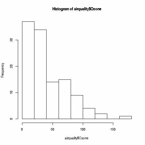
Let's do some graphics. First, remember, the columns of a data frame are vectors, so we can, for instance, plot histograms of them:
> hist(airquality$Ozone)
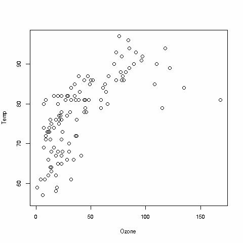
We can also draw scatter plots, say of temperature versus ozone:
> plot(airquality$Ozone,airquality$Temp)
As noted earlier for histograms, we can get fancier here, with color and so on, but let's keep it simple for now.
In our usage of plot() above, we supplied two arguments, namely the variable we wanted on the horizontal axis and the one for the vertical axis. Recall that when in Lesson 2 we called plot() on a vector, R knew to form a time-series plot for that vector. By contrast, in the above case, R knew to form a scatter plot, because we called plot() with two vector arguments. But what if we make that same call but with an entire data frame as the argument? Typing
> plot(airquality)
we get

Wow! Is R smart, or what? Seeing that we gave plot() a whole data frame, R decided that what we needed was mini-scatter plots for all possible pairs of variables in our data frame. Our plot of temperature versus ozone, for instance, is right there in the fourth row, first column.
By the way, R also provides various conveniences. For example, before doing the various operations above that had dollar signs in them, we could have issued the command:
> attach(airquality)
From that point onward, we would not need to type "airquality", e.g.
> plot(Ozone,Temp)
Programming is very much like carpentry or cooking: It is a creative activity. All the programming languages, R here, gives you is a choice of possible ingredients, such as vectors, data frames, functions and graphics--it's up to you to creatively combine those ingredients to meet your goal.
The good news is that everyone can do it. The concepts are fairly simple, and it's just a matter of reasoning out the steps needed to solve a particular problem. Don't expect to necessarily see a solution right away, and sometimes it takes some trial-and-error work. Remember my motto, "When in doubt, try it out!" I'm rather proud of inventing that motto. :-) Don't be afraid to try little experiments. And as you gain more experience, your power to apply R will continue to increase.